Introduction
Overview
Teaching: 5 min
Exercises: 0 minQuestions
What is ROOT?
What can I learn here?
Objectives
Understand what you can learn in this lesson!
Hi there, a warm welcome to the lesson about efficient analysis with ROOT!
What is ROOT?
Most likely you were already in touch with ROOT! But in short, it’s an open-source data analysis framework used by high energy physics and others, which lets you save and access your experiment’s data, allows you to process the data in a computationally efficient and statistically sound way and gives you access to all tools to produce publication-quality results.
What can I learn here?
We would like to show you how you can perform efficient data analysis with ROOT! Starting with getting access to ROOT without any hassle, you will learn the advantages of ROOT in C++ and Python. Next, we want to introduce you to a selection of features, which we see commonly used in a typical analysis. Another ingredient for efficient analysis is a simple way to get help quickly and therefore you will learn where you can find support. The last sections introduce you to the modern way to process data with ROOT and walks you through a full analysis based on CMS NanoAOD files. You can learn how to go efficiently from the initial datasets to the result plots, all powered by ROOT!
Key Points
You’ll learn how to install ROOT on your system or get access to systems with ROOT pre-installed!
You’ll learn how to use ROOT in C++ and Python!
You’ll learn about commonly used features in ROOT!
You’ll learn how to get help with ROOT!
You’ll learn to do efficient data analysis with an example based on NanoAOD files!
Get ROOT
Overview
Teaching: 10 min
Exercises: 5 minQuestions
How to install ROOT on my system or get access to systems with ROOT pre-installed?
Objectives
Find the most efficient way for you to get access to ROOT
Install ROOT or connect to a machine with ROOT already installed
This section shows you multiple ways to get ROOT. Find below solutions to run ROOT locally, on LXPLUS, in batch systems and CIs!
Conda
Conda is a package management system and environment management system, which can install ROOT in a few minutes on Linux and MacOS.
The fastes way to get ROOT is installing Miniconda (a minimal Conda installation) and then run the following two commands:
conda create -c conda-forge --name <my-environment> root
conda activate <my-environment>
You can find detailed information about ROOT on Conda in this blog post.
CVMFS
CVMFS is a software distribution service that is already set up on many HEP systems. CMSSW including ROOT is distributed via CVMFS, but also other software stacks are available that contain ROOT.
Most notably, the CERN service LXPLUS has CVMFS always installed and enables rapid access to software and computing resources.
CMSSW
The following commands let you find out quickly which ROOT version comes with CMSSW.
# Source setup tools
source /cvmfs/cms.cern.ch/cmsset_default.sh

# Show CMSSW versions
scram list

# Setup CMSSW environment (using CMSSW_11_1_3 here)
cmsrel CMSSW_11_1_3
cd CMSSW_11_1_3/

# Show information about ROOT
scram tool list | grep root

# Source this CMSSW release
cmsenv
LCG
Another option to get ROOT via CVMFS are the LCG releases. All information about the releases and contained packages can be found at http://lcginfo.cern.ch. Most releases are available as a Python 2 and Python 3 version, for example 98 and 98python3. There are also development releases every night, which contain the latest ROOT release in dev4 and the very latest developments from ROOT master in dev3.
The following example shows you how to source LCG 98 based on Python 3 on a CentOS 7 machine such as those on LXPLUS. Note the platform and compiler dependent information in the path, which have to be adjusted based on your system. The available combinations are shown on the website.
source /cvmfs/sft.cern.ch/lcg/views/LCG_98python3/x86_64-centos7-gcc10-opt/setup.sh
Docker
If you want to use ROOT in a CI system (e.g. GitLab pipelines or GitHub actions), most likely the software will be made available via Docker. The official ROOT docker containers can be found at https://hub.docker.com/r/rootproject/root. The different base images and ROOT versions are encoded in the tags, for example 6.22.00-ubuntu20.04, and latest will get you the latest ROOT release (v6.22) based on Ubuntu 20.04. If you want to try it, get Docker and run the following command to start the container with a bash shell.
docker run --rm -it rootproject/root /bin/bash
Binary releases and packages
The classic way to distribute software, besides the source code, are plain binary releases. You can download these from the release pages on https://root.cern/install/all_releases for all major MacOS and Linux versions. If you choose this installation method, make sure ROOT dependencies are installed on your system. Complete installation instructions for binary releases are available here.
In addition, for some Linux distributions, the ROOT community maintains packages in the respective package managers. You can find a list of maintained packages at https://root.cern/install/#linux-package-managers.
Verify the ROOT version
Since ROOT has a long history and numerous releases, on old systems such Scientific Linux 6 you may find correspondingly old ROOT versions. However, with the following commands you can easily verify your ROOT version and also find expert details about the ROOT configuration!
# ROOT version and build tag
root --version

# Again the ROOT version (this also works with older ROOT versions)
root-config --version

# Check that ROOT was built with C++14 support
# The output must contain one of -std=c++{14,17,1z} so that all code examples of this lesson run!
root-config --cflags

# List all the ROOT configuration options that can be checked
root-config --help
Find your way to access ROOT!
For the exercises later you need at least ROOT 6.18 and C++14 support. Feel free to set up for yourself your preferred environment satisfying this requirement!
Fallback solution
As a fallback solution you can always connect to LXPLUS via
ssh -Y your_username@lxplus.cern.ch. The-Yflag enables X forwarding, which allows you to forward the output of graphics application in case you run a system with an X server such as almost all Linux distributions.
Key Points
ROOT is accessible in several different ways
Detailed up-to-date instructions can be found at https://root.cern/install
ROOT in C++ and Python
Overview
Teaching: 10 min
Exercises: 5 minQuestions
Should I use ROOT in C++ or Python?
Objectives
Run C++ code interactively with ROOT!
Compile C++ programs using ROOT!
Use ROOT in Python!
This section shows you the difference between using ROOT with interactive C++, compiled C++ and Python.
Interactive C++
One of the main features of ROOT is the possibility to use C++ interactively thanks to the C++ interpreter Cling. Cling lets you use C++ just like Python either from the prompt or in scripts.
The ROOT prompt
By just typing root in the terminal you will enter the ROOT prompt. Like the Python prompt, the ROOT prompt is well suited to fast investigations.
$ root
root [0] 1+1
(int) 2
If you pass a file as argument to root, the file will be opened when entering the prompt and put in the variable _file0. ROOT typically comes with support for reading files remotely via HTTP (and XRootD), which we will use for the following example:
No support for remote files?
Although unlikely, your ROOT build may not be configured to support remote file access. In this case, you can just download the file with
curl -O https://root.cern/files/tmva_class_example.rootand point to your local file. No other changes required!
$ root https://root.cern/files/tmva_class_example.root
root [0]
Attaching file https://root.cern/files/tmva_class_example.root as _file0...
(TFile *) 0x555f82beca10
root [1] _file0->ls() // Show content of the file, all objects are accessible via the prompt!
TWebFile** https://root.cern/files/tmva_class_example.root
TWebFile* https://root.cern/files/tmva_class_example.root
KEY: TTree TreeS;1 TreeS
KEY: TTree TreeB;1 TreeB
root [2] TreeS->GetEntries() // Number of events in the dataset
root [3] TreeS->Print() // Show dataset structure
******************************************************************************
*Tree :TreeS : TreeS *
*Entries : 6000 : Total = 98896 bytes File Size = 89768 *
* : : Tree compression factor = 1.00 *
******************************************************************************
*Br 0 :var1 : var1/F *
*Entries : 6000 : Total Size= 24641 bytes One basket in memory *
*Baskets : 0 : Basket Size= 32000 bytes Compression= 1.00 *
*............................................................................*
*Br 1 :var2 : var2/F *
*Entries : 6000 : Total Size= 24641 bytes One basket in memory *
*Baskets : 0 : Basket Size= 32000 bytes Compression= 1.00 *
*............................................................................*
*Br 2 :var3 : var3/F *
*Entries : 6000 : Total Size= 24641 bytes One basket in memory *
*Baskets : 0 : Basket Size= 32000 bytes Compression= 1.00 *
*............................................................................*
*Br 3 :var4 : var4/F *
*Entries : 6000 : Total Size= 24641 bytes One basket in memory *
*Baskets : 0 : Basket Size= 32000 bytes Compression= 1.00 *
*............................................................................*
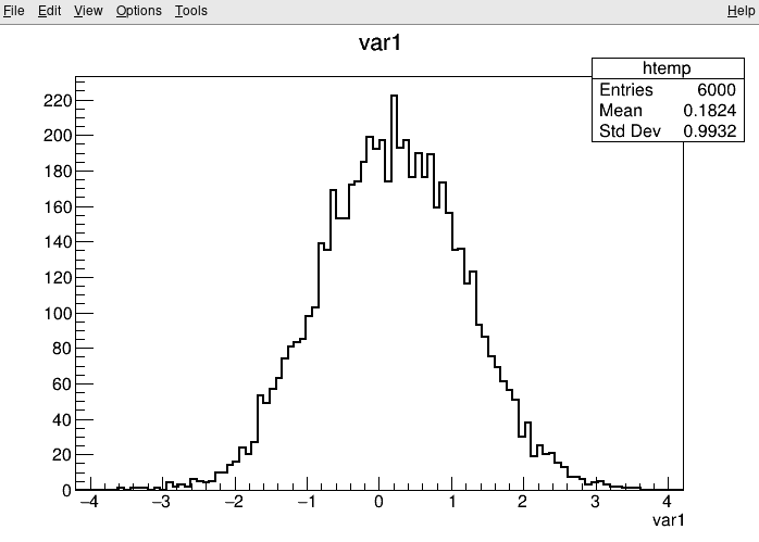
root [4] TreeS->Draw("var1") // Draw a histogram of the variable var1
ROOT scripts
A unique feature of ROOT is the possibility to use C++ scripts, also called “ROOT macros”. A ROOT script contains valid C++ code and uses as entrypoint a function with the same name as the script. Let’s take as example the file myScript.C with the following content.
void myScript() {
    auto file = TFile::Open("https://root.cern/files/tmva_class_example.root");
    for (auto key : *file->GetListOfKeys()) {
        const auto name = key->GetName();
        const auto entries = file->Get<TTree>(name)->GetEntries();
        std::cout << name << " : " << entries << std::endl;
    }
}
Scripts can be processed by passing them as argument to the root executable:
$ root myScript.C

root [0]
Processing myScript.C...
TreeS : 6000
TreeB : 6000
The advantage of such scripts is the simple interaction with C++ libraries (such as ROOT) and running your code at C++ speed with the convenience of a script.
Compiled C++
You can improve the runtime of your programs if you compile them upfront. Therefore, ROOT tries to make the compilation of ROOT macros as convenient as possible!
ACLiC
ROOT provides a mechanism called ACLiC to compile the script in a shared library and call the compiled code from interactive C++, all automatically!
The only change required to our script is that we need to include all required headers:
#include "TFile.h"
#include "TTree.h"
#include <iostream>

void myScript() {
    // The body of the myScript function goes here
}
Now, let’s compile and run the script again. Note the + after the script name!
$ root myScript.C+

root [0]
Processing myScript.C+...
Info in <TUnixSystem::ACLiC>: creating shared library /path/to/myScript_C.so
TreeS : 6000
TreeB : 6000
ACLiC has many more features, for example compiling your program with debug symbols using +g. You can find the documentation here.
C++ compilers
Of course, the C++ code can also just be compiled with C++ compilers such as g++ or clang++ with the advantage that you have full control of all compiler settings, most notable the optimization flags such as -O3!
To do so, we have to add the main function to the script, which is the default entrypoint for C(++) programs.
#include "TFile.h"
#include "TTree.h"
#include <iostream>

void myScript() {
    // The body of the myScript function goes here
}

int main() {
    myScript();
    return 0;
}
Now, you can use the following command with your C++ compiler of choice to compile the script into an executable.
$ g++ -O3 -o myScript myScript.C $(root-config --cflags --libs)
$ ./myScript
TreeS : 6000
TreeB : 6000
Computationally heavy programs and long running analyses may benefit greatly from the optimized compilation with -O3 and can save you hours of computing time!
Python
ROOT provides the Python bindings called PyROOT. PyROOT is not just ROOT from Python, but a full-featured interface to call C++ libraries in a pythonic way. This lets you import the ROOT module from Python and makes all features dynamically available. Let’s rewrite the C++ example from above and put the code in the file myScript.py!
import ROOT

rfile = ROOT.TFile.Open('https://root.cern/files/tmva_class_example.root')
for key in rfile.GetListOfKeys():
    name = key.GetName()
    entries = rfile.Get(name).GetEntries()
    print('{} : {}'.format(name, entries))
Calling the Python script works as expected:
$ python myScript.py
TreeS : 6000
TreeB : 6000
But PyROOT can do much more for you than simply providing access to C++ libraries from Python. You can also inject efficient C++ code into your Python program to speed up potentially slow parts of your program!
import ROOT

ROOT.gInterpreter.Declare('''
int my_heavy_computation(std::string x) {
    // heavy computation goes here
    return x.length();
}
''')

# Functions and object made available via the interpreter are accessible from
# the ROOT module
y = ROOT.my_heavy_computation("the ultimate answer to life and everything")
print(y) # Guess the result!
A guide to such advanced features of PyROOT can be found in the official manual at https://root.cern/manual/python. Feel free to investigate!
Try using ROOT with interactive C++, compiled C++ and Python!
Make yourself familiar with the different ways you can run an analysis with ROOT!
Key Points
The choice of interactive C++, compiled C++ or Python is based on the use case!
Usage of C++ code, compiled with optimization flags, may save you hours of computing time!
PyROOT lets you use C++ from Python but offers many more advanced features to speed up your analysis in Python. Details about the dynamic Python bindings provided by PyROOT can be found on https://root.cern/manual/python.
Commonly used features in ROOT
Overview
Teaching: 10 min
Exercises: 10 minQuestions
Which ROOT features am I likely to use in my analysis?
Objectives
Learn about important core features of ROOT
This section is dedicated to the introduction to selected features of ROOT, which we see commonly used in typical day-to-day work and analyses.
Basic histogramming, fitting and plotting
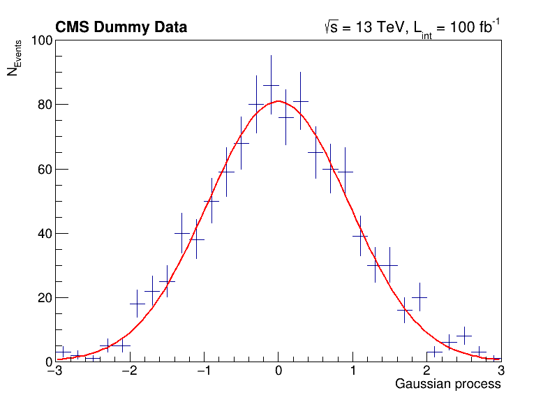
The following script uses basic features from ROOT, which are used commonly in day-to-day work with ROOT. You can investigate the typical workflow to create histograms with TH1F, fit a function to the data with TF1 and produce an accurate visualization with TCanvas and others. Below, you can see the output of the fit to the data with the measured parameters.
import ROOT
import numpy as np

# Make global style changes
ROOT.gStyle.SetOptStat(0) # Disable the statistics box
ROOT.gStyle.SetTextFont(42)

# Create a canvas
c = ROOT.TCanvas('c', 'my canvas', 800, 600)

# Create a histogram with some dummy data and draw it
data = np.random.randn(1000).astype(np.float32)
h = ROOT.TH1F('h', ';Gaussian process; N_{Events}', 30, -3, 3)
for x in data: h.Fill(x)
h.Draw('E')

# Fit a Gaussian function to the data
f = ROOT.TF1('f', '[0] * exp(-0.5 * ((x - [1]) / [2])**2)')
f.SetParameters(100, 0, 1)
h.Fit(f)

# Let's add some CMS style headline
label = ROOT.TLatex()
label.SetNDC(True)
label.SetTextSize(0.040)
label.DrawLatex(0.10, 0.92, '#bf{CMS Dummy Data}')
label.DrawLatex(0.58, 0.92, '#sqrt{s} = 13 TeV, L_{int} = 100 fb^{-1}')

# Save as png file and show interactively
c.SaveAs('dummy_data.png')
c.Draw()
 FCN=30.2937 FROM MIGRAD    STATUS=CONVERGED      67 CALLS          68 TOTAL
                     EDM=1.34686e-08    STRATEGY= 1      ERROR MATRIX ACCURATE
  EXT PARAMETER                                   STEP         FIRST
  NO.   NAME      VALUE            ERROR          SIZE      DERIVATIVE
   1  p0           8.09397e+01   3.19887e+00   7.10307e-03  -3.40988e-05
   2  p1          -3.46483e-03   3.10501e-02   8.47265e-05  -2.30742e-03
   3  p2           9.56532e-01   2.24141e-02   4.97399e-05   2.58872e-03
Info in <TCanvas::Print>: file dummy_data.png has been created
Try it by yourself!
Run the example code by yourself! In case the execution ends without displaying the plot on screen, you can run the script in interpreted mode with
python -i your_script.py. That will keep the process alive after the plot is displayed.
Investigating data in ROOT files
You have already seen the usage of TTree::Draw in the previous section. Such quick investigations of data in ROOT files are typical usecases which most analysts encounter on a daily basis. In the following you can learn about different ways to approach this task!
Manually plotting with TTree::Draw
For quick studies on the raw data in a TTree on the command line, you can use TTree::Draw to make simple visualizations:
$ root https://root.cern/files/tmva_class_example.root
root [0]
Attaching file https://root.cern/files/tmva_class_example.root as _file0...
(TFile *) 0x558d7b54aa50
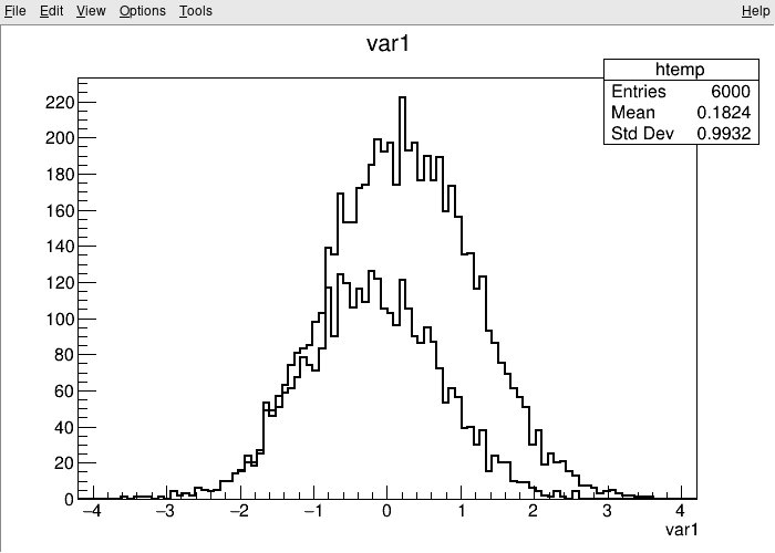
root [1] TreeS->Draw("var1") // just draw var1
Info in <TCanvas::MakeDefCanvas>: created default TCanvas with name c1
root [2] TreeS->Draw("var1", "var2 > var1", "SAME") // draw var1 with the selection var2 > var1
(long long) 3222
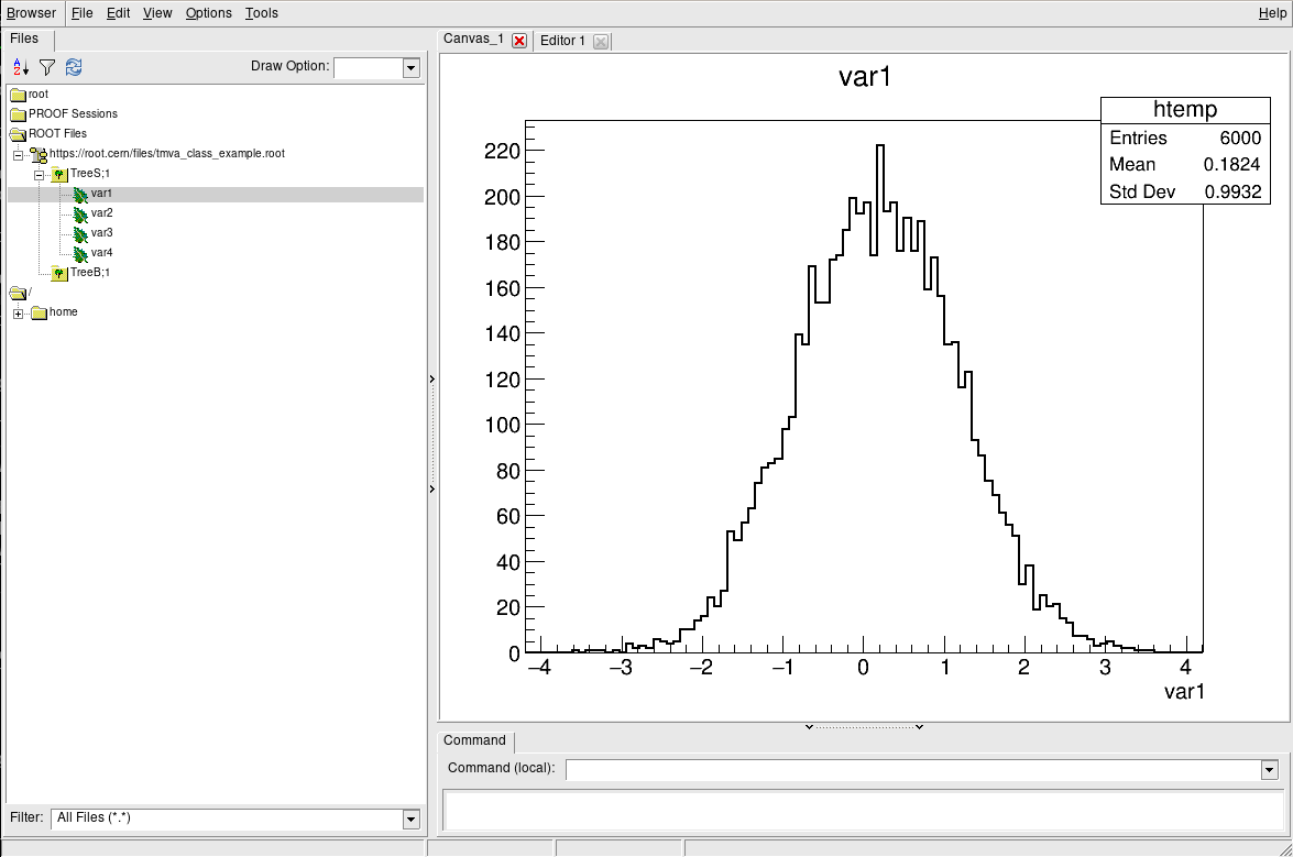
The TBrowser
More convenient is using ROOT’s tool for browsing ROOT files, the TBrowser. You can spawn the GUI directly from the ROOT prompt as shown below.
$ root https://root.cern/files/tmva_class_example.root

root [0]
Attaching file https://root.cern/files/tmva_class_example.root as _file0...
(TFile *) 0x557892a0ef10
root [1] TBrowser b
(TBrowser &) Name: Browser Title: ROOT Object Browser
The rootbrowse executable
For convenience, ROOT provides the executable rootbrowse, which lets you open a TBrowser directly from the command line and display the files given as arguments!
$ rootbrowse https://root.cern/files/tmva_class_example.root
Other ROOT executables
There are many small helpers shipped with ROOT, which let you operate on data quickly from the command line and solve typical day-to-day tasks with ROOT files.
List of ROOT executables
rootbrowse: Open a ROOT file and a TBrowserrootls: List file content, tree branches, objects’ statsrootcp: Copy objects within a file or between filesrootdrawtree: Simple analyses from the command linerooteventselector: Select branches, events, compression algorithms and extract slimmer treesrootmkdir: Creates a directory in a TFilerootmv: Move objects between filesrootprint: Print objects in plots on filesrootrm: Remove objects from files
$ rootls https://root.cern/files/tmva_class_example.root
TreeB  TreeS
$ rootls -l https://root.cern/files/tmva_class_example.root
TTree  Jan 19 14:25 2009 TreeB  "TreeB"
TTree  Jan 19 14:25 2009 TreeS  "TreeS"
$ rootls -t https://root.cern/files/tmva_class_example.root
TTree  Jan 19 14:25 2009 TreeB  "TreeB"
  var1    "var1/F"    0
  var2    "var2/F"    0
  var3    "var3/F"    0
  var4    "var4/F"    0
  weight  "weight/F"  0
  Cluster INCLUSIVE ranges:
   - # 0: [0, 5998]
   - # 1: [5999, 5999]
  The total number of clusters is 2
TTree  Jan 19 14:25 2009 TreeS  "TreeS"
  var1  "var1/F"  0
  var2  "var2/F"  0
  var3  "var3/F"  0
  var4  "var4/F"  0
  Cluster INCLUSIVE ranges:
   - # 0: [0, 5998]
   - # 1: [5999, 5999]
  The total number of clusters is 2
Try it by yourself!
Feel free to investigate the tools presented here!
Interoperability with NumPy arrays
There are many reasons, for example machine learning applications, to want to export your data in Python to NumPy arrays. This is easily possible with ROOT and is part of RDataFrame. The code snippets below show you how to do this conversion and how to move the data to typical tools in the Python ecosystem, e.g., numpy and pandas.
numpy and pandas
Have you installed
numpyandpandasor are you on a system which has them available? Normally, you can just runpip install --user numpy pandasto install missing packages! Another option is searching in your system package manager, they are typically available on all platforms.
Convert data in ROOT files to numpy arrays
The conversion feature is attached to the class RDataFrame. We will not introduce you here to this way to process data with ROOT because the following section is dedicated to RDataFrame. For now, just keep in mind that you call AsNumpy! The data is returned as a dictionary of one-dimensional numpy arrays.
# Read out the data as a dictionary of numpy arrays
import ROOT
df = ROOT.RDataFrame('TreeS', 'https://root.cern/files/tmva_class_example.root')
columns = ['var1', 'var2', 'var3', 'var4']
data = df.AsNumpy(columns)
print('var1: {}'.format(data['var1']))
var1: [-1.1436108 2.1434433 -0.44391322 ... 0.37746507 -2.072639 -0.09141494]
Move the data to numpy or pandas
The data can be passed naturally to any method in the Python ecosystem which processes numpy arrays. Below is an example that computes the mean of each column.
# Apply numpy methods
import numpy as np
print('Means: {}'.format([np.mean(data[c]).item() for c in columns]))
Means: [0.18244409561157227, 0.28425973653793335, 0.3789360225200653, 0.7712161540985107]
Another interesting usecase is moving the dataset directly to a pandas dataframe. You can use the output of AsNumpy directly as input to its constructor.
# Convert to a pandas dataframe
import pandas
pdf = pandas.DataFrame(data)
print(pdf)
          var1      var2      var3      var4
0    -1.143611 -0.822373 -0.495426 -0.629427
1     2.143443 -0.018923  0.267030  1.267493
2    -0.443913  0.486827  0.139535  0.611483
3     0.281100 -0.347094 -0.240525  0.347208
4     0.604006  0.151232  0.964091  1.227711
...        ...       ...       ...       ...
5995 -0.040650 -0.154212 -0.097715  0.440331
5996  0.099931 -1.183759  0.034616  0.644502
5997  0.377465 -0.030945  1.166082  0.728614
5998 -2.072639 -0.635586 -0.747371 -1.285679
5999 -0.091415  0.221271  0.569032  1.386130

[6000 rows x 4 columns]
Try it by yourself!
The statements are very short, you can just copy paste them into the Python prompt. Feel free to investigate what you can do with
AsNumpy! Further information can be found here.
ROOT in Jupyter notebooks
ROOT provides a deep integration with Jupyter notebooks. You can start a Jupyter notebook server including ROOT features with the following command:
root --notebook
Alternatively, you can go to https://swan.cern.ch, which provides Jupyter notebooks integrated with CERN’s cloud storage as a web service. Note that you may have to visit https://cernbox.cern.ch first at least once with your user account to create your CERNBox space!
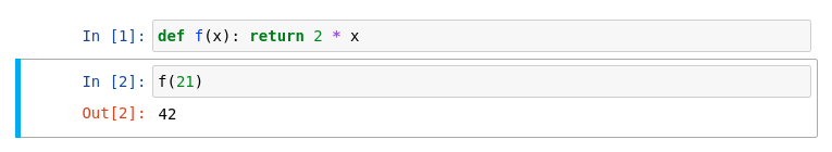
Python kernel
Jupyter is often use to edit Python code interactively. By creating a new notebook with a Python kernel, you will see something similar to the screenshot below and you can work interactively with Python in the browser!
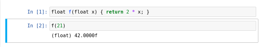
C++ kernel
ROOT provides a Jupyter C++ kernel, which behaves similarly to the Python kernel but for C++! Similar to the ROOT prompt, you can work interactively with C++ in the notebook. Just select the C++ kernel in the drop-down menu!
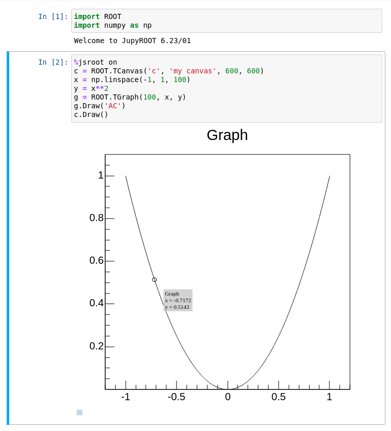
JSROOT
Another feature of ROOT is the %jsroot on magic, which enables ROOT’s JavaScript integration! This allows you to interact with the visualization such as you are used to it from the interactive graphics in the Python prompt.
Because it’s JavaScript, we can also embed these plots easily in any website. You can find an interactive version of the plot from the top of this section at the bottom of the page. For example, you can zoom in, add grid lines or get detailed information about the data points, right here!
Try it by yourself!
Either run Jupyter locally via
root --notebookor go to https://swan.cern.ch to try ROOT in a Jupyter notebook!
More useful features
ROOT is made for HEP analysis and contains many other features that are useful in typical tasks, for example:
- TEfficiency, to handle histograms representing efficiencies and their uncertainties
- THStack, to stack histograms
- TRatioPlot, to create ratio plots with the histograms on the top and the ratio with the correct uncertainties on the bottom
- And many more!
Key Points
ROOT provides many features from histogramming, fitting and plotting to investigating data interactively in C++ and Python
Efficient analysis with RDataFrame
Overview
Teaching: 10 min
Exercises: 5 minQuestions
How can I perform efficient analysis with ROOT?
Objectives
Learn about the basics of RDataFrame
Understand RDataFrame’s lazy event loop feature
Find out how to run your analysis on multiple threads
What is RDataFrame?
RDataFrameis ROOT’s high-level interface for efficient data analysis. WithRDataFrame, it is possible to read, select, modify and write ROOT data, as well as easily produce histograms, cut-flow reports and other results. In this and the following sections, you will learn how to perform data analysis withRDataFrame, running all your tasks efficiently on multiple threads!
Download the dataset
Most likely, you will run multiple times over the used dataset with a size of 2.1 GB. To speed up the process, please download the file upfront. Either go to http://opendata.web.cern.ch/record/12341 and click the download button at the bottom or use the command below.
xrdcp root://eospublic.cern.ch//eos/opendata/cms/derived-data/AOD2NanoAODOutreachTool/Run2012BC_DoubleMuParked_Muons.root .
Implicit multi-threading in ROOT
ROOT tries to make parallelization as simple as possible for you. For this reason, we offer the feature ROOT.EnableImplicitMT(N), which enables thread safety for the relevant classes and runs parallelized parts of ROOT, such as RDataFrame, implicitely on N threads:
import ROOT

# Enable multi-threading with the specified amount of threads (let's start with just one)
# Note that older ROOT versions may require to write ROOT.ROOT.EnableImplicitMT()
ROOT.EnableImplicitMT(1)

# Or enable multi-threading with an auto-detected amount of threads
#ROOT.EnableImplicitMT()
RDataFrame constructor and Filter transformations
A possible way to construct an RDataFrame is passing one (ore more) filepaths and the name of the dataset (i.e. the name of the TTree object in the file, which is called Events in this section).
Next, you can apply selections and other transormations to the dataframe. The first basic transformation is applying cuts with the Filter method. Note that each transformation returns a new, transformed dataframe and does not change the dataframe object itself!
# Create dataframe from a (reduced) NanoAOD file
df = ROOT.RDataFrame("Events", "Run2012BC_DoubleMuParked_Muons.root")

# For simplicity, select only events with exactly two muons and require opposite charge
df_2mu = df.Filter("nMuon == 2", "Events with exactly two muons")
df_os = df_2mu.Filter("Muon_charge[0] != Muon_charge[1]", "Muons with opposite charge")
Injection of C++ code and Define transformations
The next code block uses PyROOT to inject a C++ implementation of the invariant mass computation. The name of the just-in-time compiled function can be used in the Define method to add a new column to the dataset, which will contain the dimuon mass.
# Compute invariant mass of the dimuon system

# Perform the computation of the invariant mass in C++
ROOT.gInterpreter.Declare('''
using Vec_t = const ROOT::RVec<float>&;
float ComputeInvariantMass(Vec_t pt, Vec_t eta, Vec_t phi, Vec_t mass) {
    const ROOT::Math::PtEtaPhiMVector p1(pt[0], eta[0], phi[0], mass[0]);
    const ROOT::Math::PtEtaPhiMVector p2(pt[1], eta[1], phi[1], mass[1]);
    return (p1 + p2).M();
}
''')

# Add the result of the computation to the dataframe
df_mass = df_os.Define("Dimuon_mass", "ComputeInvariantMass(Muon_pt, Muon_eta, Muon_phi, Muon_mass)")
Booking results
At any point, you can book the computation of results, e.g., histograms or a cut-flow report. Both of them are added below. Please note that RDataFrame is lazy! This means that the computation does not run right away, when you book a histogram, but you can accumulate multiple results and compute all of them in one go. The computation of all booked results is triggered only when you actually access one of the results!
# Book histogram of the dimuon mass spectrum (does not actually run the computation!)
h = df_mass.Histo1D(("Dimuon_mass", ";m_{#mu#mu} (GeV);N_{Events}", 30000, 0.25, 300), "Dimuon_mass")

# Request a cut-flow report (also does not run the computation yet!)
report = df_mass.Report()
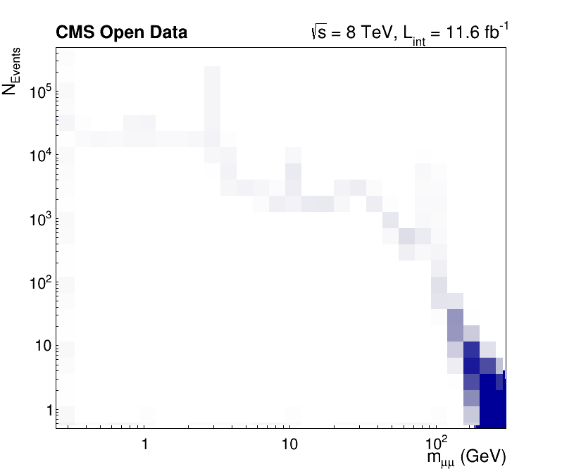
Computing the result and making a plot
As explained above, accessing a dataframe result triggers the computation (sometimes called “event loop”) of all results booked up to that point. Here, this happens when we access the axis of the histogram. However, you just have to remember to book all results first and then start working with the results so that they can all be computed in one go! At the end, we also print the cut-flow report to investigate the efficiency of the filters.
# Produce plot
ROOT.gStyle.SetOptStat(0)
ROOT.gStyle.SetTextFont(42)
c = ROOT.TCanvas("c", "", 800, 700)
# The contents of one of the dataframe results are accessed for the first time here:
# this is when all results will actually be produced!
h.GetXaxis().SetTitleSize(0.04)
h.GetYaxis().SetTitleSize(0.04)
c.SetLogx(); c.SetLogy()
h.Draw()

label = ROOT.TLatex()
label.SetNDC(True)
label.SetTextSize(0.040)
label.DrawLatex(0.100, 0.920, "#bf{CMS Open Data}")
label.DrawLatex(0.550, 0.920, "#sqrt{s} = 8 TeV, L_{int} = 11.6 fb^{-1}")

# Save as png file
c.SaveAs("dimuon_spectrum.png")

# Print cut-flow report
report.Print()
Events with exactly two muons: pass=31104343   all=61540413   -- eff=50.54 % cumulative eff=50.54 %
Muons with opposite charge: pass=24067843   all=31104343   -- eff=77.38 % cumulative eff=39.11 %
Run the code by yourself to get a high-resolution dimuon spectrum, which shows resonances from 250 MeV to 300 GeV!
Try it by yourself!
- Assemble the code pieces and compute a high-resolution dimuon spectrum in under one minute!
- Note that you have to keep the Python interpreter running to investigate the plot interactively. You can do this with
python -i your_script.py- Does the computation time decrease with an increasing number of threads
NinROOT.EnableImplicitMT(N)?- Could you name the resonances?
Key Points
RDataFrameis the recommended entry point for efficient analysis
RDataFrameis lazy: declare first what you want to do and let ROOT run all of your tasks as efficiently as possible in one go, in parallel!Parallelization on multiple threads requires only the
ROOT.EnableImplicitMT()statement
How to get help with ROOT?
Overview
Teaching: 10 min
Exercises: 0 minQuestions
Where can I find documentation?
Where can I ask for help?
Objectives
Learn how to find the official documentation!
Learn about the ROOT forum to get help!
Something does not work as expected, how can I get help?
User support is an integral part of ROOT and happily provided by the ROOT team!
We provide multiple communication channels so that we can help you but also you can help yourself to find the right answers to your questions, as fast as possible!
Support and discussion channel for this lesson
Communication channels for support and discussion dedicated to this lesson are linked on the front page!
The ROOT website, the beginner’s guide and the manual
The ROOT website is home to the beginner’s guide and the more in-depth manual. These are a great resource to start with ROOT and learn about parts of the framework in high detail. Keep in mind the ROOT website at https://root.cern, which provides links to all resources in a single place!
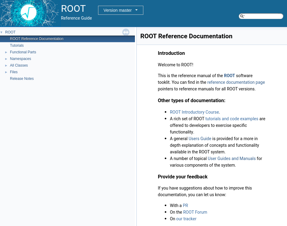
The reference guide
The reference guide provides a more technical documentation about ROOT powered by Doxygen. You can search for classes or functions in ROOT, learn about types and methods and trace features down to the actual implementation.
Although the reference guide is more technical in first place, important classes have extensive additional documentation. Feel free to investigate TTree or RDataFrame!
Another part of the reference guide are the tutorials, which explain features in working code examples. Feel free to look at tutorials for RooFit and RDataFrame, which cover many typical use cases for these parts of ROOT!
The ROOT forum
The ROOT forum is the to-go place if you cannot find the answer in the documentation. Don’t hesitate to open a discussion, there is always someone from the ROOT team actively taking care of new questions in the forum!
But not only questions are very welcome, you can also discuss possible improvements or make suggestions for new features!

Bug tracking
Bugs are currently tracked on Jira, but we will soon switch to GitHub issues. However, if you discover bugs, please report them! In case you are not sure whether you see a bug or a feature, posting in the ROOT forum is always a good idea and always appreciated!
Key Points
User support is an integral part of ROOT!
https://root.cern is the entry point to find all documentation
The reference guide provides in-depth technical documentation, but also additional explanation for classes and a huge amount of tutorials explaining features with code
The ROOT forum is actively maintained by the ROOT team to support you!
Well done, take a break!
Overview
Teaching: min
Exercises: minQuestions
Objectives

Key Points
NanoAOD analysis: Introduction
Overview
Teaching: 10 min
Exercises: 10 minQuestions
What am I supposed to learn from this analysis?
What is the physics behind the data?
Objectives
Learn the basics of the physics processes present in the data
Learn about the content of the (reduced) NanoAOD files
The following sections show you how an analysis with CMS NanoAOD files and RDataFrame can be performed, from the inital files to the result plots.
Signal process
The physical process of interest, also often called signal, is the production of the Higgs boson in the decay to two tau leptons. The main production modes of the Higgs boson are the gluon fusion and the vector boson fusion production indicated in the plots with the labels gg→H and qq→H, respectively. See below the two Feynman diagrams that describe the processes at leading order.


Tau decay modes
The tau lepton has a very short lifetime of about 290 femtoseconds after which it decays into other particles. With a probability of about 20% each, the tau lepton decays into a muon or an electron and two neutrinos. All other decay modes consist of a combination of hadrons such as pions and kaons and a single neutrino. You can find here a full overview and the exact numbers. This analysis considers only tau lepton pairs of which one tau lepton decays into a muon and two neutrinos and the other tau lepton hadronically, whereas the official CMS analysis considered additional decay channels.
Background processes
Besides the Higgs boson decaying into two tau leptons, many other processes can produce very similar signatures in the detector, which have to be taken into account to draw any conclusions from the data. In the following, the most prominent processes with a similar signature as the signal are presented. Besides the QCD multijet process, the analysis estimates the contribution of the background processes using simulated events.
Z→ττ
The most prominent background process is the Z boson decaying into two tau leptons. The leading order production is called the Drell-Yan process in which a quark anti-quark pair annihilates. Because the Z boson decays directly into two tau leptons, same as the Higgs boson, this process is very hard to distinguish from the signal.
Z→ll
Besides the decay of the Z boson into two tau leptons, the Z boson decays with the same probability to electrons and muons. Although this process does not contain any genuine tau leptons, a tau can be reconstructed by mistake. Objects that are likely to be misidentified as a hadronic decay of a tau lepton are electrons or jets.
W+jets
W bosons are frequently produced at the LHC and can decay into any lepton. If a muon from a W boson is selected together with a misidentified tau from a jet, a similar event signature as the signal can occur. However, this process can be strongly suppressed by a cut in the event selection on the transverse mass of the muon and the missing energy, as done in the published CMS analysis.
tt¯
Top anti-top pairs are produced at the LHC by quark anti-quark annihilation or gluon fusion. Because a top quark decays immediately and almost exclusively via a W boson and a bottom quark, additional misidentifications result in signal-like signatures in the detector similar to the $W+\mathrm{jets}$ process explained above. However, the identification of jets originating from bottom quarks, and the subsequent removal of such events, is capable of reducing this background effectively.
QCD
The QCD multijet background describes decays with a large number of jets, which occurs very often at the LHC. Such events can be falsely selected for the analysis due to misidentifications. Because a proper simulation of this process is complex and computational expensive, the contribution is not estimated from simulation but from data itself. Therefore, we select tau pairs with the same selection as the signal, but with the modified requirement that both tau leptons have the same charge. Then, all known processes from simulation are subtracted from the histogram. Using the resulting histogram as estimation for the QCD multijet process is possible because the production of misidentified tau lepton candidates is independent of the charge.
Files and dataset content
The used files and the content of the datasets, for example the simulated Standard Model Higgs boson produced by Gluon fusion, can be found on the CERN Open Data portal.
Have a look at the content of the (reduced) CMS NanoAOD files!
You can just look at the content on the CERN Open Data portal (follow for example this link) or take one of the files you will download below and investigate the content with ROOT, such as shown in the previous sections!
Why NanoAOD?
The NanoAOD format is a small version of the MiniAOD format (which is a small version of the AOD format) with a size of about 1 kB/Event. Going towards Run 3 and 4 of the LHC, this format will be very likely the default for most CMS analyses to be able to process an unprecedented amount of data!
Why reduced NanoAOD?
Note that the used NanoAOD files are reduced versions recreated with open CMS data and simulation from 2012, but you will most likely not see any difference!
Download the required datasets
Because very likely you will run the code multiple times, we want to speed up the analysis so that you can focus on the software. To do so, download with xrdcp the files on your computer or any other system with ROOT (v6.18 or later) available. The size of downloaded files sum up to about 6.5 GB and represent only 10% of the original files you can find on the Open Data portal, which enables you to run the full analysis in under five minutes.
Alternatively, you can download the files manually via HTTP from https://root.cern/files/HiggsTauTauReduced/.
SAMPLES=(
    GluGluToHToTauTau
    VBF_HToTauTau
    DYJetsToLL
    TTbar
    W1JetsToLNu
    W2JetsToLNu
    W3JetsToLNu
    Run2012B_TauPlusX
    Run2012C_TauPlusX
    )

for SAMPLE in ${SAMPLES[@]}
do
    # Via XRootD:
    xrdcp root://eospublic.cern.ch//eos/root-eos/HiggsTauTauReduced/${SAMPLE}.root .
    # Via HTTP:
    # curl -O https://root.cern/files/HiggsTauTauReduced/${SAMPLE}.root
done
Download the files!
Choose one of the options shown above and download the files!
Key Points
Analysis studies Higgs boson decays to two tau leptons with a muon and a hadronic tau in the final state
The input files are (reduced) CMS NanoAOD, being very close to actual analysis in CMS
The following steps will show in a hands-on the use of RDataFrame in an actual analysis
NanoAOD analysis: Skim the initial datasets
Overview
Teaching: 5 min
Exercises: 10 minQuestions
How can I process large amounts of data efficiently?
How does an analysis with RDataFrame look like in C++?
Objectives
Perform this step of the analysis by yourself
In this step, the NanoAOD files containing data and simulated events are pre-processed. This step is called skimming since the event selection reduces the size of the datasets significantly. In addition, we perform a pair selection to find from the muon and tau collections the pair which is most likely to have originated from a Higgs boson.
This step is implemented in the file skim.cxx here and is written in C++ for performance reasons.
Download the code and investigate the content!
Download the file
skim.cxxand investigate the content. You can easily follow the steps in themainfunction!
Compile the C++ program!
Compile the file
skim.cxxto an executable!Note that you require ROOT built with C++14 or later. You can find out by looking at the output of
root-config --cflags, which must contain-std=c++14or-std=c++17!
Compile the C++ program!
Use the following command and replace
g++with the C++ compiler of your choice.g++ -O3 -o skim skim.cxx $(root-config --cflags --libs)
Run the C++ program and investigate the output!
Run it! Note that the program picks up the files from the same directory in which you run it. Also the results of this step are files in the same directory in which you have run the executable and have the filenames
*Skim.root.
Have you noticed the ROOT::RVec class?
ROOT::RVec is an extended std::vector with additional features to deal with collections, similar to NumPy arrays. Because RVec has the same interface as a std::vector you can use them interchangeably! However, following additional features simplifies typical tasks in analysis. You can find the full documentation here!
Note that all vectors in RDataFrame are automatically treated as RVecs. You can use all features shown below in strings passed to RDataFrame!
Adopting memory
You can adopt memory just by passing the pointer and the length of the vector! This may improve the runtime of your program greatly because copies are costly operations.
// Adopting memory
int d[3] = { 1, 2, 3 };
ROOT::RVec<int> v(d, 3); // { 1, 2, 3 }
Arithmetic operations and masking
You can use arithmetic operations and masking with RVecs, just like with NumPy arrays!
// Arithmetic operations
ROOT::RVec<int> x = { 1, 2, 3 };
auto y = pow(x, 2); // { 1, 4, 9 }
auto z = x + y; // { 2, 6, 12 }
// Masking
ROOT::RVec<int> x = { 0, 1, 2 };
ROOT::RVec<int> y = { 1, 2, 3 };
auto z = y[x > 0]; // { 2, 3 }
NumPy-like helper functions
// Sorting, index manipulation, comparison, ...
using namespace ROOT::VecOps;
RVec<int> x = { 3, 1, 2 };
auto y = Reverse(Sort(x)); // { 3, 2, 1 }
auto idx = Argsort(x); // { 1, 2, 0 } (the indices sorting the vector x)
auto z = Take(x, idx); // { 1, 2, 3 } (the sorted vector)
auto allEqual = All(Reverse(z) == y); // true (compares all elements)
ROOT::VecOps also offers helpers typical to HEP such as DeltaPhi and InvariantMass. You can find working code examples explaining these helpers in the VecOps tutorials!
Try it by yourself!
Feel free to open the ROOT prompt and try
ROOT::RVecby yourself! The prompt is well suited to try some of the features shown above because you can print the content of the vectors just by leaving out the semicolon at the end of the line.
Key Points
We reduced the initial datasets by filtering suitable events and selecting interesting observables.
This step includes finding the interesting muon-tau pair in each selected event.
To perform this computationally expensive part of the analysis as efficiently as possible, we enable ROOT’s implicit multi-threading and use RDataFrame in C++!
ROOT::RVecis an extendedstd::vector, which provides features to deal easily with collections similar to NumPy arrays in Python.
NanoAOD analysis: Produce histograms
Overview
Teaching: 5 min
Exercises: 5 minQuestions
How to produce many histograms efficiently?
How does an analysis with
RDataFramelook like in Python?Objectives
Produce all histograms required for the final plots
Understand why we need so many histograms for a single plot
In the previous section, we produced skimmed datasets from the original files but still preserved information of selected quantities for each event. In this step, we compute histograms of these quantities for all skimmed datasets. Because of the data-driven QCD estimation, similar histograms have to be produced with the selection containing same-charged tau lepton pairs. This sums up to multiple hundreds of histograms which have to be combined into the final plots such as the ones shown in the next section.
For convenience, this step is implemented in Python in the file histograms.py, which you can download here.
Investigate and run the Python script!
Have a look at the code and run it! Note that the program picks up the files from the same directory in which you run it.
Investigate the output!
The script produces the file
histograms.root, which contains the histograms. You can have a look at the plain histograms using for example the ROOT browser!
Key Points
We produce histograms of all physics processes and all observables.
All histograms are produced in a signal region with opposite-signed muon-tau pairs and in a control region with same-signed pairs for the data-driven QCD estimate
This step shows the usage of RDataFrame in Python producing a large number of histograms in a single event loop and in parallel!
NanoAOD analysis: Make the plots
Overview
Teaching: 5 min
Exercises: 5 minQuestions
How can I make high quality plots with ROOT?
Objectives
Make plots of all observables
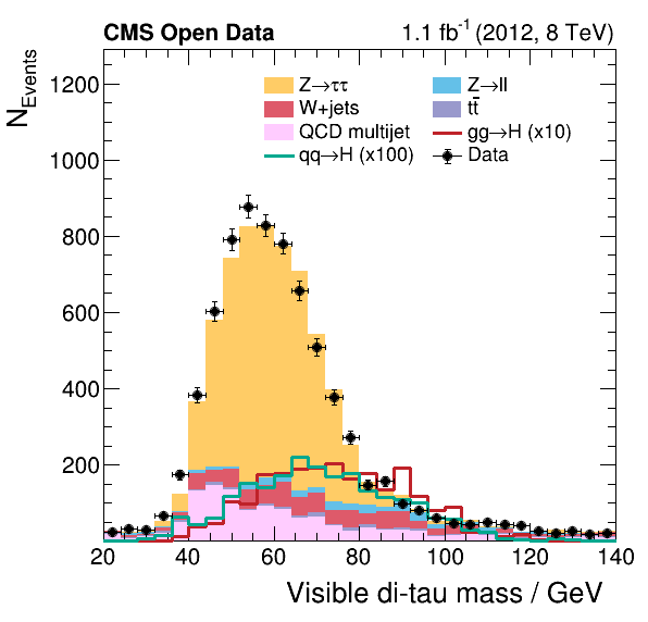
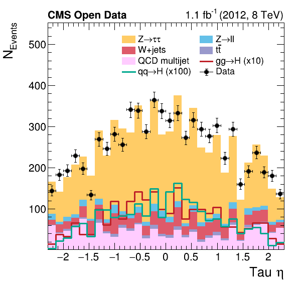
Finally, the histograms we produced in the previous section are combined to produce the final plots showing the data taken with the CMS detector compared with the expectation from the background estimates. These plots allow one to study the contribution of the different physics processes to the data taken with the CMS detector and represent the first step towards verifying the existence of the Higgs boson.
This step is again implemented in Python for convenience and can be found in the file plot.py, which you can download here.
Investigate and run the Python script!
Have a look at the code and run it! Note again that the program picks up the files from the same directory in which you run it.
Investigate the output!
The Python script generates a
pngand a
Key Points
The plotting combines all histograms to produce estimates of the physical processes and create a figure with a physical meaning.
The plots show the share of the contributing physical processes to the data, but without systematic uncertainties.
The script shows how you can produce paper quality plots with ROOT!
Success, you finished!
Overview
Teaching: min
Exercises: minQuestions
Objectives

Key Points