Commonly used features in ROOT
Overview
Teaching: 10 min
Exercises: 10 minQuestions
Which ROOT features am I likely to use in my analysis?
Objectives
Learn about important core features of ROOT
This section is dedicated to the introduction to selected features of ROOT, which we see commonly used in typical day-to-day work and analyses.
Basic histogramming, fitting and plotting
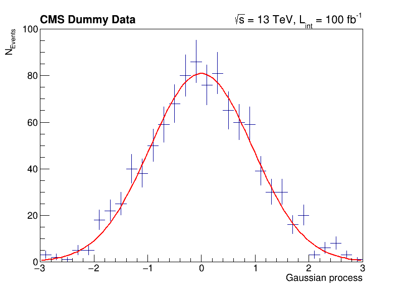
The following script uses basic features from ROOT, which are used commonly in day-to-day work with ROOT. You can investigate the typical workflow to create histograms with TH1F, fit a function to the data with TF1 and produce an accurate visualization with TCanvas and others. Below, you can see the output of the fit to the data with the measured parameters.
import ROOT
import numpy as np

# Make global style changes
ROOT.gStyle.SetOptStat(0) # Disable the statistics box
ROOT.gStyle.SetTextFont(42)

# Create a canvas
c = ROOT.TCanvas('c', 'my canvas', 800, 600)

# Create a histogram with some dummy data and draw it
data = np.random.randn(1000).astype(np.float32)
h = ROOT.TH1F('h', ';Gaussian process; N_{Events}', 30, -3, 3)
for x in data: h.Fill(x)
h.Draw('E')

# Fit a Gaussian function to the data
f = ROOT.TF1('f', '[0] * exp(-0.5 * ((x - [1]) / [2])**2)')
f.SetParameters(100, 0, 1)
h.Fit(f)

# Let's add some CMS style headline
label = ROOT.TLatex()
label.SetNDC(True)
label.SetTextSize(0.040)
label.DrawLatex(0.10, 0.92, '#bf{CMS Dummy Data}')
label.DrawLatex(0.58, 0.92, '#sqrt{s} = 13 TeV, L_{int} = 100 fb^{-1}')

# Save as png file and show interactively
c.SaveAs('dummy_data.png')
c.Draw()
 FCN=30.2937 FROM MIGRAD    STATUS=CONVERGED      67 CALLS          68 TOTAL
                     EDM=1.34686e-08    STRATEGY= 1      ERROR MATRIX ACCURATE
  EXT PARAMETER                                   STEP         FIRST
  NO.   NAME      VALUE            ERROR          SIZE      DERIVATIVE
   1  p0           8.09397e+01   3.19887e+00   7.10307e-03  -3.40988e-05
   2  p1          -3.46483e-03   3.10501e-02   8.47265e-05  -2.30742e-03
   3  p2           9.56532e-01   2.24141e-02   4.97399e-05   2.58872e-03
Info in <TCanvas::Print>: file dummy_data.png has been created
Try it by yourself!
Run the example code by yourself! In case the execution ends without displaying the plot on screen, you can run the script in interpreted mode with
python -i your_script.py. That will keep the process alive after the plot is displayed.
Investigating data in ROOT files
You have already seen the usage of TTree::Draw in the previous section. Such quick investigations of data in ROOT files are typical usecases which most analysts encounter on a daily basis. In the following you can learn about different ways to approach this task!
Manually plotting with TTree::Draw
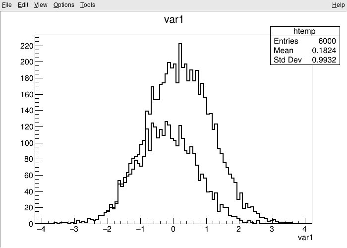
For quick studies on the raw data in a TTree on the command line, you can use TTree::Draw to make simple visualizations:
$ root https://root.cern/files/tmva_class_example.root

root [0]
Attaching file https://root.cern/files/tmva_class_example.root as _file0...
(TFile *) 0x558d7b54aa50
root [1] TreeS->Draw("var1") // just draw var1
Info in <TCanvas::MakeDefCanvas>:  created default TCanvas with name c1
root [2] TreeS->Draw("var1", "var2 > var1", "SAME") // draw var1 with the selection var2 > var1
(long long) 3222
The TBrowser
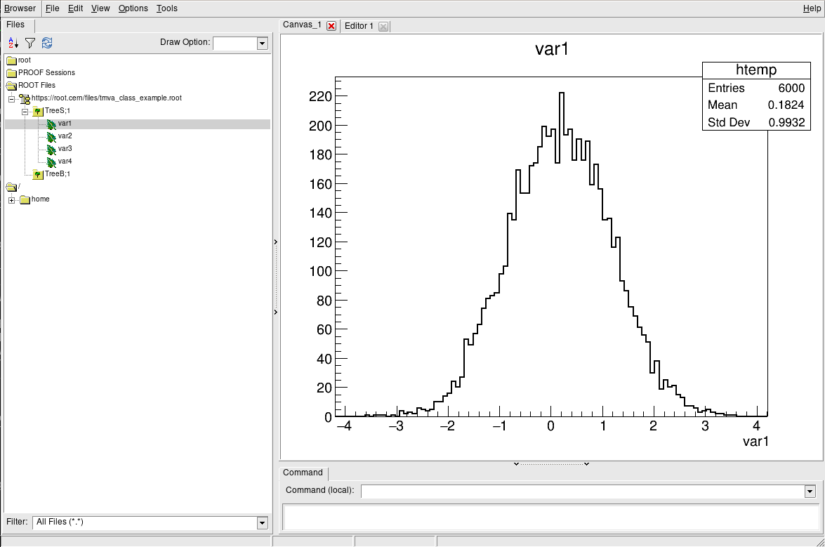
More convenient is using ROOT’s tool for browsing ROOT files, the TBrowser. You can spawn the GUI directly from the ROOT prompt as shown below.
$ root https://root.cern/files/tmva_class_example.root

root [0]
Attaching file https://root.cern/files/tmva_class_example.root as _file0...
(TFile *) 0x557892a0ef10
root [1] TBrowser b
(TBrowser &) Name: Browser Title: ROOT Object Browser
The rootbrowse executable
For convenience, ROOT provides the executable rootbrowse, which lets you open a TBrowser directly from the command line and display the files given as arguments!
$ rootbrowse https://root.cern/files/tmva_class_example.root
Other ROOT executables
There are many small helpers shipped with ROOT, which let you operate on data quickly from the command line and solve typical day-to-day tasks with ROOT files.
List of ROOT executables
rootbrowse: Open a ROOT file and a TBrowserrootls: List file content, tree branches, objects’ statsrootcp: Copy objects within a file or between filesrootdrawtree: Simple analyses from the command linerooteventselector: Select branches, events, compression algorithms and extract slimmer treesrootmkdir: Creates a directory in a TFilerootmv: Move objects between filesrootprint: Print objects in plots on filesrootrm: Remove objects from files
$ rootls https://root.cern/files/tmva_class_example.root
TreeB  TreeS
$ rootls -l https://root.cern/files/tmva_class_example.root
TTree  Jan 19 14:25 2009 TreeB  "TreeB"
TTree  Jan 19 14:25 2009 TreeS  "TreeS"
$ rootls -t https://root.cern/files/tmva_class_example.root
TTree  Jan 19 14:25 2009 TreeB  "TreeB"
  var1    "var1/F"    0
  var2    "var2/F"    0
  var3    "var3/F"    0
  var4    "var4/F"    0
  weight  "weight/F"  0
  Cluster INCLUSIVE ranges:
   - # 0: [0, 5998]
   - # 1: [5999, 5999]
  The total number of clusters is 2
TTree  Jan 19 14:25 2009 TreeS  "TreeS"
  var1  "var1/F"  0
  var2  "var2/F"  0
  var3  "var3/F"  0
  var4  "var4/F"  0
  Cluster INCLUSIVE ranges:
   - # 0: [0, 5998]
   - # 1: [5999, 5999]
  The total number of clusters is 2
Try it by yourself!
Feel free to investigate the tools presented here!
Interoperability with NumPy arrays
There are many reasons, for example machine learning applications, to want to export your data in Python to NumPy arrays. This is easily possible with ROOT and is part of RDataFrame. The code snippets below show you how to do this conversion and how to move the data to typical tools in the Python ecosystem, e.g., numpy and pandas.
numpy and pandas
Have you installed
numpyandpandasor are you on a system which has them available? Normally, you can just runpip install --user numpy pandasto install missing packages! Another option is searching in your system package manager, they are typically available on all platforms.
Convert data in ROOT files to numpy arrays
The conversion feature is attached to the class RDataFrame. We will not introduce you here to this way to process data with ROOT because the following section is dedicated to RDataFrame. For now, just keep in mind that you call AsNumpy! The data is returned as a dictionary of one-dimensional numpy arrays.
# Read out the data as a dictionary of numpy arrays
import ROOT
df = ROOT.RDataFrame('TreeS', 'https://root.cern/files/tmva_class_example.root')
columns = ['var1', 'var2', 'var3', 'var4']
data = df.AsNumpy(columns)
print('var1: {}'.format(data['var1']))
var1: [-1.1436108 2.1434433 -0.44391322 ... 0.37746507 -2.072639 -0.09141494]
Move the data to numpy or pandas
The data can be passed naturally to any method in the Python ecosystem which processes numpy arrays. Below is an example that computes the mean of each column.
# Apply numpy methods
import numpy as np
print('Means: {}'.format([np.mean(data[c]).item() for c in columns]))
Means: [0.18244409561157227, 0.28425973653793335, 0.3789360225200653, 0.7712161540985107]
Another interesting usecase is moving the dataset directly to a pandas dataframe. You can use the output of AsNumpy directly as input to its constructor.
# Convert to a pandas dataframe
import pandas
pdf = pandas.DataFrame(data)
print(pdf)
          var1      var2      var3      var4
0    -1.143611 -0.822373 -0.495426 -0.629427
1     2.143443 -0.018923  0.267030  1.267493
2    -0.443913  0.486827  0.139535  0.611483
3     0.281100 -0.347094 -0.240525  0.347208
4     0.604006  0.151232  0.964091  1.227711
...        ...       ...       ...       ...
5995 -0.040650 -0.154212 -0.097715  0.440331
5996  0.099931 -1.183759  0.034616  0.644502
5997  0.377465 -0.030945  1.166082  0.728614
5998 -2.072639 -0.635586 -0.747371 -1.285679
5999 -0.091415  0.221271  0.569032  1.386130

[6000 rows x 4 columns]
Try it by yourself!
The statements are very short, you can just copy paste them into the Python prompt. Feel free to investigate what you can do with
AsNumpy! Further information can be found here.
ROOT in Jupyter notebooks
ROOT provides a deep integration with Jupyter notebooks. You can start a Jupyter notebook server including ROOT features with the following command:
root --notebook
Alternatively, you can go to https://swan.cern.ch, which provides Jupyter notebooks integrated with CERN’s cloud storage as a web service. Note that you may have to visit https://cernbox.cern.ch first at least once with your user account to create your CERNBox space!
Python kernel
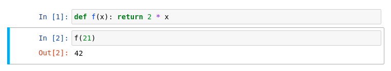
Jupyter is often use to edit Python code interactively. By creating a new notebook with a Python kernel, you will see something similar to the screenshot below and you can work interactively with Python in the browser!
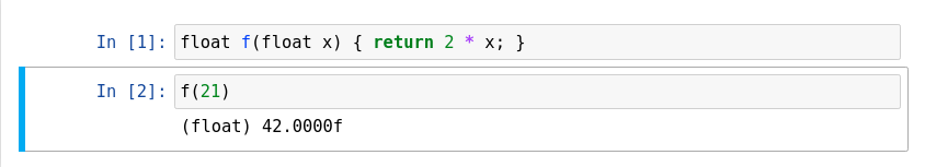
C++ kernel
ROOT provides a Jupyter C++ kernel, which behaves similarly to the Python kernel but for C++! Similar to the ROOT prompt, you can work interactively with C++ in the notebook. Just select the C++ kernel in the drop-down menu!
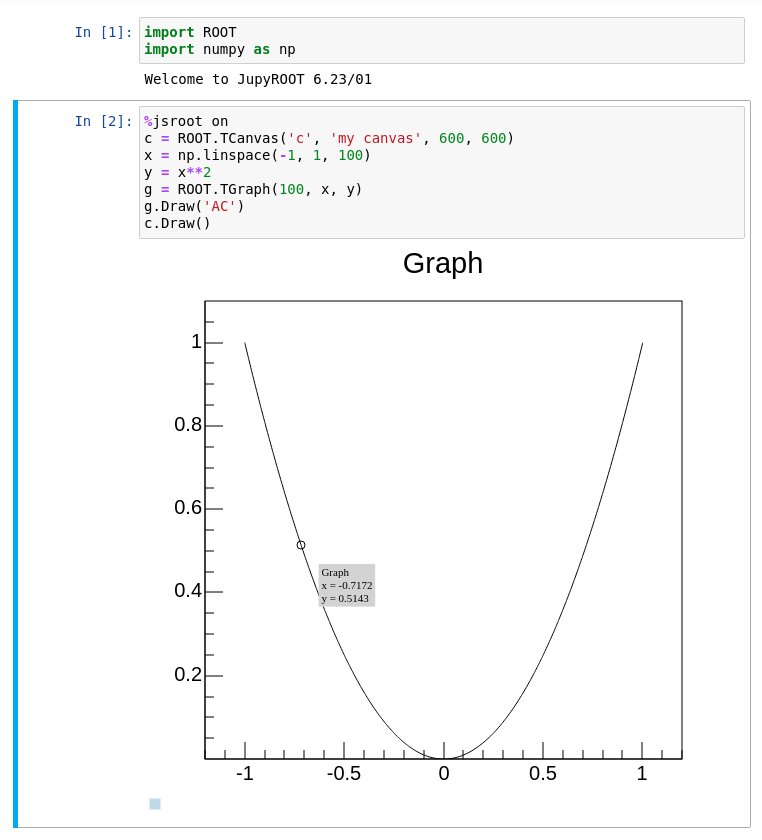
JSROOT
Another feature of ROOT is the %jsroot on magic, which enables ROOT’s JavaScript integration! This allows you to interact with the visualization such as you are used to it from the interactive graphics in the Python prompt.
Because it’s JavaScript, we can also embed these plots easily in any website. You can find an interactive version of the plot from the top of this section at the bottom of the page. For example, you can zoom in, add grid lines or get detailed information about the data points, right here!
Try it by yourself!
Either run Jupyter locally via
root --notebookor go to https://swan.cern.ch to try ROOT in a Jupyter notebook!
More useful features
ROOT is made for HEP analysis and contains many other features that are useful in typical tasks, for example:
- TEfficiency, to handle histograms representing efficiencies and their uncertainties
- THStack, to stack histograms
- TRatioPlot, to create ratio plots with the histograms on the top and the ratio with the correct uncertainties on the bottom
- And many more!
Key Points
ROOT provides many features from histogramming, fitting and plotting to investigating data interactively in C++ and Python