Wednesday DAS Plenary 10-11h
Overview
Teaching: 70 min
Exercises: 0 minQuestions
Objectives
From 10h00-11h10 there will be a DAS Plenary, please tune in to that.
Key Points
Here is a link to the indico page for Wednesday’s plenary.
Introduction to All-Hadronic b*->tW and Useful Tools
Overview
Teaching: 30 min
Exercises: 20 minQuestions
Who are the facilitators and team members?
What is this exercise about, and what should we expect from the next few days?
Why search for heavy resonances?
What is version control and CI/CD?
Objectives
Familiarize ourselves with peers and resources.
Contexualize a CMS-style search and its stages
Understand motivation for physics at high masses/scales.
Begin developing new habits with good coding practices.
Introductions
First we can begin with some introductions. The facilitators are:
- Johan Sebastian Bonilla Castro, Postdoc at the University of California – Davis, they work on all-hadronic VLQ and ttbar resonance searches as well as CSC upgrades.
- Lucas Corcodilos, Graduate Student at John Hopkins University, he works on an all-hadronic b*->tW search.
- John C. Hakala, Postdoc at the University of Virginia, he works on a leptophobic Z’ cascade decay search.
- Brendan Regnery, Graduate Student at the University of California – Davis, he works on an all=hadronic VLQ search and GEM upgrades.
The team members are:
- Elham Khazaie, PhD student at Isfahan University of Technology, Iran, working on the search for an exotic decay of the Higgs boson, also working on Luminosity Calibration.
- Davide Bruschini, Master’s Student at the University of Pisa - Currently working on the search for EW photon+2 jets events (VBF to photon) at CMS
- Elham Khazaie, PhD student at Isfahan University of Technology, Iran, working on the search for an exotic decay of the Higgs boson, also working on Luminosity Calibration.
- Florian Eble, PhD student at ETH Zurich, working on Dark Matter search by looking for Semi-Visible Jets, also working on luminosity in BRIL.
- Yusuf Can Cekmecelioglu, Masters Student at Bogazici Univeristy, Istanbul – Currently working on back-end of the HGCal detector.
- Federica Riti, PhD student at ETH Zurich, she works on the search for lepton flavour universality violation via the R(J/psi) measurement.
- Kaustuv Datta, PhD student at ETH Zurich, working on measurements of bases of N-subjettiness observables to map out the phase space of emissions in light jets, and jets originating from boosted W boson and top quark decays.
- Jongwon Lim, PhD student at Hanyang University, Republic of Korea, working on searching for lepton flavour violation in top quark sector with charm, muon, and tau final states.
The overall goal of this long exercise is to offer everyone a high-level exposure of the different components of a physics analysis. In practice, carrying out an analysis takes months and often past a year; we hope to cover the key points of the process and won’t have too much time to do so. To help you through the material, we will be providing some useful code for your use. We strongly suggest you focus on understanding the conceptual flow of the analysis and to ask as many questions as you’d like. We also encourage that you get creative and challenge yourself! If there are any parts of the exercise that you feel you can tackle by writing your own scripts, or optimizing ours, please do! We are all collaborators and we can learn a lot from each other.
Using Git
Before moving on, let’s all get on the same page and test that our workspaces have the packages they need. In the above menu bar, click on Setup and follow the instructions there.
Next, fork+clone the exercise’s repositories. Bookmark the website GitHub repository and the code repository on GitLab. When you navigate to both of these websites, click on the ‘Fork’ button towards the top-right of the page. (You will need to be logged into your GitHub/GitLab accounts)
Question: What is the difference between GitHub and GitLab
You may have noticed that the code repositories hosting the tutorial info and the analysis code used in this exercise use different services (GitHub vs GitLab). Why is this the case?
Solution
GitHub is completely public, whereas GitLab is maintained by CERN and requires credential to host projects. Depending on the needs of the project you are working on, you may want the public nature of GitLab or the speciic tools of GitLab. For example, GitLab’s CI/CD has additional features that are specifically useful to developing analysis software.
Include instructions on how to make sure environment is good to go
Now that you have forked the code onto your personal project space, let’s clone your repository onto your working directory and while we’re at it also set the upstreams:
ssh -Y <LPCUsername>@cmslpc-sl7.fnal.gov
cd ~/nobackup
mkdir CMSVDAS2020
git clone https://github.com/<GitHubUsername>/b2g-long-exercise.git <nameYourTutorialPackage>
cd <nameYourTutorialPackage>
git remote add upstream https://github.com/CMSDAS/b2g-long-exercise.git
git remote -v
cd ..
git clone https://gitlab.cern.ch/<GitLabUsername>/b2g-long-exercise-code.git <nameYourCodePackage>
cd <nameYourCodePackage>
git remote add upstream https://gitlab.cern.ch/cms-b2g/b2g-long-exercise-code.git
git remote -v
cd ..
ls .
Now our code is ready to be worked on.
Good Software Development Habits
Let’s take a few minutes to think about working on software projects as a colloboration. The code you run today (and tomorrow) has been developed by thousands of folks like you trying to make everyone’s life slightly easier. You will probably spend a lot of time reading other people’s code and will quickly build a standard on what ‘good code’ looks like. Similarly when working as a group on a common piece of software, we find good and bad ways to make changes.
To combat these problems, we agree to have a set of ‘good-practices’ for keeping software clean and easy to interpret. First, is the use of comments. When developing a script, begin by stating the code’s intended purpose and a general roadmap to the file. For each function you define (and also important data structures), include in-line comments explaining clearly what the functions/objects are used for. When making commits and merge requests on git, add detailed comments (think about having to sort through dozens of undescribed commits months after pushing them).
Version control is a way of tracing the history of software projects by recording changes encoded in ‘commits/pushes’. We will be using GitHub and CERN’s GitLab to develop our code. CI/CD (Continuous Integrationa and Deployment) is a technique for developing tests on changes (pushes) to the repository. One can, for example, create a test that compiles the code and returns and error if it cannot; one can also create tests for enforcing code style, or execute sample runs of analysis code. The sky is the limit for how fancy you want to make your CI/CD. What do you think should be implemented for our code?
“Homework” (, or bonus part of the lesson)
You should have already forked and cloned your personal version of the repository generating this website. By forking the repository, you have made your own copy of the code which generates a copy of this website, which means you have a tutorial website of your own! (Assuming you haven’t already developed a website with GitHub) To check out your website, go to https://GitHubUsername.github.io/b2g-long-exercise/
In the introduction section at the top of the lesson, you may remember there was a ‘TBA’ space in the (empty) list of participants. The goal of the following execise is to populate that list with brief introductions to you all, by changes you make to your local fork that you will then request to merge into the main website.
The general steps to follow here are:
- (Before developing) Ensure the code you have is up-to-date with
cd ~/nobackup/CMSVDAS2020/<nameYourTutorialPackage>
git fetch --all
<Enter credentials, (if any) new branches/tags will be made available>
git merge upstream gh-pages
git checkout -b <nameNewBranch>
git branch -v
<Develop code>
git status
git add <fileChanged>
git commit -m 'Write a message describing change'
git push -u origin <nameNewBranch>
<Make Merge(Pull) Request through browser onto main b2g-long-exercises repo>
- (If already developed, but changes in upstream branch) You may have to rebase your changes on top of upstream commit.
cd ~/nobackup/CMSVDAS2020/<nameYourTutorialPackage>
<Previous code development>
git branch -v
<If no branch created> git checkout -b <nameNewBranch>
git status
git add <fileChanged>
git commit -m 'Write a message describing change'
git fetch --all
<Enter credentials, new branches/tags are made available>
git rebase upstream gh-pages
git push -u origin <nameNewBranch>
<Make Merge(Pull) Request through browser onto main b2g-long-exercises repo>
Check your websites to make sure the changes look like what you want, it may take a few minutes for the build to update on the site. You can request a pull request through your repository page on GitHub. Before finishing this part of the episode, make sure all repositories are up to date and have the correct latest commit:
cd ~/nobackup/CMSVDAS2020/<nameYourTutorialPackage>
git remote -v
git branch -v
If you do not feel comfortable with git yet, that is ok. This is a learning experience and what we hope you get out of this is being conviced that proper use of versioning is useful when working in a collaboration like CMS. Ask your facilitators for help if you feel stuck, whatever the problem may be, the point of these exercises is to give you ‘big picture’ experiences not coding challenges.
The All-Hadronic b*->tW final state
The b* resonance is a beyond the standard model (BSM) particle that can be produced at the LHC when a b-quark from the incoming proton’s quark-sea interacts with a gluon from the other proton to form an excited resonance that decays to a top-quark and W-boson. The top quark almost always decayse to t->b+W, thus in the final state we have a jet from a b-decay with the W decay jets from the top and the prompt W from the b* decay. It is then the decay channels of the W bosons that determine the final state of the process. In this exercise we will focus on the all-hadronic channel.
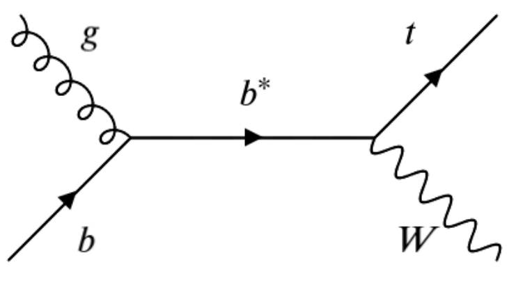
In upcoming episodes we will investigate in detail the topology of our signal, as well as possible background standard model (SM) processes that we must model and estimate their expected rates for our search.
Key Points
First level of help is at peer-level. The facilitators are here to help for any issues you are unsure about.
The big picture is: analyses begin with a motivating final state, then we optimize some selections to keep signal and reject background, finally we consider all systematic uncertainties associated with our selections and modeling in order to quantify the observations we make. Each stage of this process needs dedicated studies and may be performed individually or as a larger team.
The LHC and experiments are preparing for Run 3 and HL-LHC; we are exploring models that are motivated by exclusions/measurements made by Run 2 observations.
Eliminate fear-of-losing-data by using version control! Commit often, and document, document, document. Save yourself time later by setting CI/CD tests.
Friday DAS Plenary 10-11h
Overview
Teaching: 30 min
Exercises: 0 minQuestions
Objectives
From 10-11h there will be a DAS Plenary, please tune in to that.
Key Points
Here is a link to the indico page for Friday’s plenary.
Diving into jet substructure
Overview
Teaching: 20 min
Exercises: 40 minQuestions
What is jet substructure?
What does the jet substructure look like for the signal?
What are some commonly used jet substructure observables for t/W identification?
How can jet substructure help combat background and differentiate it from signal?
Objectives
Familiarisation with common jet substructure variables.
Identify possible discriminating variables for b*->tW signal.
Jets
After collision, colored particles (with a lifetime longer than the hadronization time scale, i.e. not tops) form cone-like hadronic showers as they propagate away from the interaction point. In experiment, we can only see the interactions of the ‘stable’ particles (pions, kaons, etc.) with the detectors, which are on average 2/3 charged particles. The calorimeters measure the energy deposits of these partilces, but we have to decide how to combine those energy deposits to best reconstruct the final state partons. In CMS, we use the Particle Flow technique to define PF candidates which we then cluster into jets.
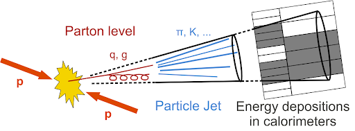
When analyzing hadronic final states, it is important to understand the jet collections used to cluster energy deposited by the hadronic showers of the final state quarks and gluons. The most common jet clustering algorithm, anti-kt, groups together ‘softer’ (low kT) objects onto harder (high kT) objects recursively until all objects are separated by a distance of the input R-parameter; the R-parameter of a jet defines the maximum radius that it can cluster constituents into itself. Normally, we use R=0.4 to define single-parton jets, e.g. low pT top decays into three separate (resolved) jets.
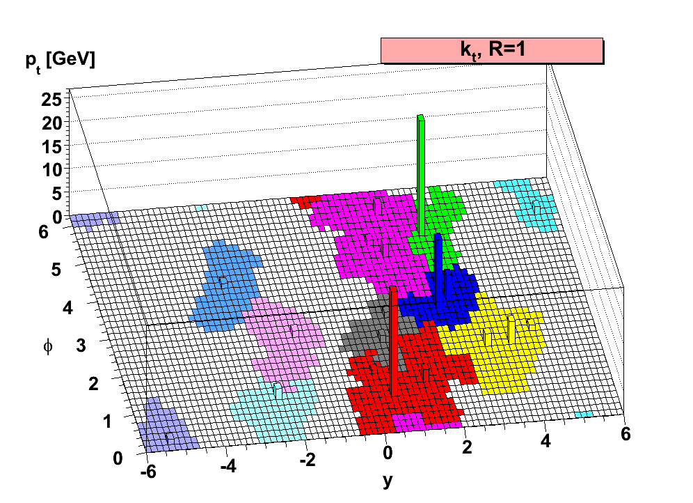
Sometimes, we want to capture the entire decay of a heavy object using a larger-R jet. The R-parameter used for these puposes depends on the mass and transverse momentum of the decaying particle, and tends to be between R=0.8-1.2. A good rule of thumb is that the opening angle of a massive particle decaying into much lighter constituents is R<2m/pT.
Question: What is are the opening angles for 200 GeV tops? What about 200 GeV Ws? What if they are at high pT ~ 1TeV?
Solution
The useful expression here is R<2m/pT. For a 200 GeV top, R<346/200 -> R<1.73. At the same transverse momentum, a W opens at R<160/200 -> R<0.8. At 1 TeV, the top decays in a cone of about R<0.35 and for the 1 TeV W it is R<0.16. As you may notice, high pT heavy (boosted) objects tend to be well encapsulated by R=0.8 jets. But, at very high pT the decaying objects are quite columnated. The choice of R-parameter for your jet collection, in a way, defines the lower bound of the pT you are sensitive to.
Jet Substructure
Jet substructure is a family of analysis techniques that studies the detailed structure within jets through the constituents of the object. When we cluster PF candidates into anti-kt jets, we can keep the information of which PF candidate is associated with which anti-kt jet. Afterwards, we can calculate substructure observables with the stored information.
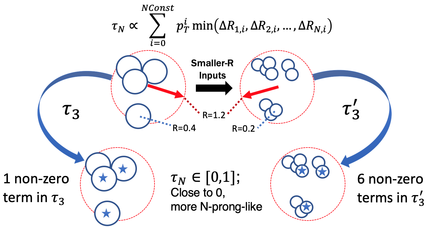
- N-Subjetiness (τN) is a set of observables that quantifies how N-pronged a jet looks like. The definition is in the image below, and it is essentially a pT-weighted moment of the constituent objects with respect to the closest of N subjets. There are many possible ways to defend where the N subjets are to be centered, but the most common is the N highest pT constituents. The observable is normalized such that the observable is always between [0,1] and the closer the result is to 0 the more N-pronged the jet is. Link to paper
- τ32/τ21 is an observable made my taking the ratio of 3-subjetiness to 2-subjetiness (2-subjetiness to 1-subjetiness). &tau32 asks the question how much more 3-pronged vs 2-pronged does this jet look like; τ21 asks the question how much more 2-pronged vs 1-pronged does this jet look like. For top decays, we would expect low τ32, whereas for W decays are expected to have a low value of τ21.
- Energy Correlation Functions are similar to the previous observable in the sense that is uses information from the constituent objects to form an observable to differentiate boosted objects from QCD multi-jet objects. However, it does not require defining subjets, as it defines the observable through pair-wise angles and the energies of the contituents. The closer the value is to 0, the more structure is present in the object. Link to paper
- Softdrop mass is not quite a traditional substructre variable, but it is commonly used in conjunction with the above. Soft-drop is a technique of jet grooming, in which constituents of a jet are removed depending on their momenta and distance from the jet’s centroid. The assumption is that soft radiation, far from the jet axis, is not likely to be part of the hard parton hadronization and thus dropped. Link to paper
- b-discriminant: another not-so-traditional substructure variable that quantifies how likely a jet (or its constituents) contains a b-hadron. This is done by evaluating the secondary vertex information, impact parameters, and other observables that try to identify a b-hadron decay. The higher the number, the more likely it is to contain a b-hadron.
Tops decay (almost always) to b+W, and since we are looking at the all-hadronic channel we are dealing with a W that decays to two quarks. Tagging an all-hadronic top is looking for a 3-pronged jet, where one of those prongs has the decay products of a b-hadron, and typically also requiring the presence of a b-hadron decay and a jet mass close to the 173 GeV of the top quark. W bosons are tagged as two pronged jets in a mass window around 80 GeV.
Question: What jet substructure observables do you think could be used to identify our signal?
Solution
Since we are looking for both a W and a top, we should consider the jet mass. Since our jets will have prong-ed structure, we should consider the N-subjetiness ratios τ32 and τ21. In addition, we can use the impact parameter information (through the form of CSV).
Another way to utilize the constituent information of jets is through the use of Machine Learning models. Below are brief descriptions of some taggers developed within CMS:
- BEST: Multiclassifiers of heavy objects. Boosts PF candidates along jet axis and defines ‘Boosted Event Shape’ variables to be evaluated on a NN. (WIP: jet images in W/Z/H/t rest frames)
- deepAK8: Multiclasifier of heavy objects. Takes low-level PF candidate and tracking information as input to deep NN.
- ImageTop: Clasifies all=hadronic top decays. Uses the topology of the PF candidates by making jet images and evaluating them with a CNN.
- ParticleNet: Utilizes a point-cloud approach to representing the PF candidates (as opposed to pixels). Has been shown to classify tops and serve as a quark/gluon discriminant.
Exercise
Use the time before the lunch break to look into the signal sample provided. One quick way to check out its contents is to open the file in interactive root (turning on bash mode with -b helps open the application faster)
root -b /eos/home-l/lcorcodi/Storage/rootfiles/BprimeLH1200_bstar16.root
.ls
_file0->Print()
When loaded from start-up, the file is assigned the ‘_file0’ variable; dig into the information available and see what is available for you to use. Try using the plotting script provided to see some distributions:
cd ~/CMSVDAS2020/CMSSW_11_0_1/src/
cmsenv
cd timber-env
source timber-env/bin/activate
cd ../TIMBER
source setup.sh
cd ../BstarToTW_CMSDAS2020
python exercises/ex4.py -y 16
The very last line calls on the plotting script, and it is using some root files we have already made for y’all. If you would like to change the selections and make the plots, make the appropriate chages to the script and run it with an additional ‘–select’ flag.
Try adding your plots to the B2G-Long-Exercise website through the _extras/figures.md file.
Key Points
Jet substructure are analysis techniques for measuring a jet observable through its constituent information.
N-subjetiness is how ‘N-pronged’ a jet looks, more specifically for N subjets it is the sum of pt-weighted constuent-subjet spatial moments.
Traditional top-tagging typically uses τ32 and jet mass, whereas for W-tagging it’s τ21 and the jet mass.
Investigating the signal topology
Overview
Teaching: 5 min
Exercises: 25 minQuestions
What is the signal we are trying to select for?
What observables should be investigated for our final state?
What do kinematics in the signal look like?
How do observables change as a function of resonance mass?
Is there an observable that directly probes the signal?
Objectives
Familiarisation with the ntuple format.
Plot several kinematic variables at parton, particle, and reconstructed level. (Bonus: Investigate relative resolution)
Reconstruct the invariant resonance mass.
One of the first questions we should ask ourselves is ‘what does our signal look like?’ Understanding the answer to this will help us decide what selections we should apply to keep as much of the signal as we can, while rejecting as much background as possible. Before making any decisions, we should open up the signal sample we have and get ourselves acquainted with what information is available to us. Sometimes, samples are ‘slimmed’ (removal of unnecessary infomation/branches) or ‘skimmed’ (application of loose selections to reduce number of events) in order to reduce the size of the sample files.
To check the information inside a sample, open it up with root and checkout it’s branches
root -b xrdcp root://cmsxrootd.fnal.gov//eos/store/lcorcodilos/samples/signal.root
.ls
myTree->Print()
myTree->Scan("JetPt")
myTree->Scan("JetPt","JetPt<400")
myTree->Scan("JetPt","JetPt<300")
myTree->Draw("JetPt")
There are more sophisticated ways to investigate the branches available as well as their min/max values in root and python.
Question: Can you find any previous selections that have been applied to the signal sample? If so, why do you think they were done?
Solution
The jet pT has been required to be 350 GeV, and the absolute value of the jet eta (|η|) is 2.5.
Bonus Exercises:
Write a python script that reads the signal sample and outputs each branch name along with the min/max value of that branch into a txt file. Write a pyRoot script that reads the signal sample and outputs plots of each branch, using the min/max values you found above in the binning definition.
You may notice that some variables appear in several variations, e.g. JetPt, PFcandsPt, truthTopPt. What are the different types of collections available (reconstructed, particle, parton, truth, etc.)?
Bonus++: Plot the relative resolutions of the reconstructed objects you have with respect to their truth values. For example, the relative resolution of jet transverse momentum is JER=(recoJetPt-truthJetPt)/truthJetPt
Finally, let’s look into one of the most important observables of the signal: the effective mass of the t+W system.
Key Question
What does this effective mass mean? Does it represent anything physical? Before plotting, what do you think the distribution should look like, and why?
Key Points
In an all-hadronic state, we veto leptons (electrons/muons) and study jet properties.
Jets are clustered Particle Flow candidates interpreted as a 4-vector with momenta, energy, and mass.
The resonance searched decays to all particles in final state, thus if we add all jets in vector-form we can reconstruct the resonance.
Friday Lunch 12-13h
Overview
Teaching: 0 min
Exercises: 60 minQuestions
Objectives
Enjoy your lunch from 12-13h :)
Key Points
Developing a pre-selection
Overview
Teaching: 10 min
Exercises: 50 minQuestions
What is the purpose of a preselection?
What loose cuts could you apply that follow the signal topology?
What are background processes that could enter this selection?
How do I normalise background processes?
Objectives
Define a ‘good’ region of the detector and apply MET filters.
Develop a simple signal selection cutflow.
Make stack plots of background processes.
Recording files of this session are in cernbox
Introduction
A preselection serves two purposes, first to ensure that passing events only utilize a “good” region of the detector with appropriate noise filters and second to start applying simple selections motivated by the physics of the signal topology.
Defining a “Good” Region of the Detector
A “good” region of the detector depends heavily on the signal topology. The muon system and tracker extend to about |η| = 2.4 while the calorimeter extends to |η| = 3.0 with the forward calorimeter extending further. Thus, if the signal topology relies heavily on tracking or muons, then a useful preselection would limiting the region to |η| < 2.4. Some topologies, like vector boson fusion (commonly called VBF) have two forward (high eta) jets, so placing a preselection that requires two forward jets is a useful preselection.
Discuss (5 min)
Now, let’s take a more detailed look at our signal topology and see how it fits in with the detector. The b-star is produced from the interaction of a bottom quark and a gluon, will this production mode yield any characteristic forward jets? In this topology, the b-star decays to a jet from a W boson and a jet from a top quark. What is characteristic of a top jet? What about a W jet? How does this impact the region of the detector needed? What |η| and φ in the detector do we need? Think about this while looking at the Feynman diagram and the signal topology.
Solution
The production mode does not have any characteristic forward jets, but the final state has two jets. The top quark decays to a b jet and W jet, where the b jet is typically identified by making use of it’s characteristic secondary vertex. This secondary vertex is identified in the tracker. Both the W jet and top jet have unique substructure that can be used to distinguish them from QCD jets. Therefore it is crucial to use a region of the detector with good tracking and granular calorimetery,so we should restrict |η| < 2.4. There are no detector differences in phi that should impact this search, so there should be no restriction in φ.

Finding Appropriate MET Filters
Missing transverse momentum (called MET) is used to identify detector noise and MET filters are used to remove detector noise. The MET group publishes recommendations on the filters that should be used for different eras of data.
Exercise (5 min)
The recommended MET filters for Run II are listed on this twiki. Use this twiki to create a list of MET filters to use in the preselection.
Simple Selections
The preselection should also include a set of simple selections based on our physics knowledge of the signal topology. These “simple” selections typically consist of loose lower bounds only, which help to reduce the number of events which will get passed to the rest of the analysis while still preserving the signal region.
Consider a heavy resonance decaying to two Z bosons that produce jets to create a dijet final state. In this case, the energy of the collision would go into producing a heavy resonance with little longitudinal momentum, so conservation of momentum tells us that the jets should be well separated in φ, ideally they should have a separation of π in φ. Therefore placing a selection of Δφ > π/2 should not cut out signal, but will reduce the number of events passed on to the next stage.
Reflect
Why not use a selection close to Δφ = π?
Solution
The jets can recoil off of other objects creating a dijet pair that is less than Δφ = π
This also a good stage to place a lower limit on the jet pT. In a hadronic analysis, it is common to place a high lower limit on the pT. For this example, a lower limit of pT = 400 GeV should be good.
Reflect
Why place such a high lower limit on jet pT?
Solution
This is a tricky question. It relates to the trigger. Hadronic triggers have a turn on at high HT or high pT, so the lower limit ensures that that the analysis will only investigate the fully efficient region.
A jet originating from a Z boson should also have two “prongs” (regions of energy in the calorimeter), these “prongs” are part of the jet substructure discussed in the earlier lessons. For a two pronged jet like a Z jet, it is good to place a lower limit on the τ21 ratio. Another useful substructure variable to use in the preselection is the softdrop mass. The softdrop algorithm will help to reduce the amount of pileup that is used when measuring the jet mass. The preselection is a good place to define a wide softdrop mass region. For this example, a wide region around the Z boson mass would be ideal, such as 65 < mSD < 115 GeV.
It is important to emphasize that the preselections should be relatively light. It is important to check that the preselection is not eliminating large amounts of signal. A good way to monitor this is to utilize stacked histograms. More about these plots is described below.
Discuss (5 min)
Again, use the images above to think about the signal topology. What “simple” selections can be used in the preselection? Any Δφ or pT criteria? What about substructure?
Solution
In this signal topology the t and W should be well separated, so a light Δφ cut should be placed. Think about a reasonable selection and investigate the result in the plotting exercise. Same for the jet pT. Both the top jet and the W jet should have substructure. The top jet should have three prongs and W jet should have two prongs. Think about the softdrop regions and n-subjettiness (τ) ratios that should be used and investigate them in the plotting exercise.
Applying our selection and monitoring the MC response
When applying the preselection, the selections will be placed serially in the code creating a “cutflow”. The filters are applied first to ensure that the data was taken in “good” detector conditions. Then the kinematic/substructure cuts are applied. It is important to monitor the signal and background in between these physics inspired cuts.
Exercise (20 min) Plots to Monitor Signal and Background
Find where the filters are applied in the
exercises/ex4.pyscript, check that all the filters are there, and then create a histogram displaying τ21 τ32 for the leading and subleading jet. This can be done using theexercises/ex4.pyscript from theBstarToTW_CMSDAS2020repository.cd CMSSW_11_0_1/src # where you saved the TIMBER and BstarToTW_CMSDAS2020 repositories during the setup cmsenv python -m virtualenv timber-env source timber-env/bin/activate python exercises/ex4.py -y 16 --selectWhat criteria would you use for τ21? What about τ32?
Solution
The filters are listed as flags
flags = ["Flag_goodVertices",
       "Flag_globalTightHalo2016Filter",
       "Flag_eeBadScFilter",
       "Flag_HBHENoiseFilter",
       "Flag_HBHENoiseIsoFilter",
       "Flag_ecalBadCalibFilter",
       "Flag_EcalDeadCellTriggerPrimitiveFilter"]
Then they are applied using the
Cutfunction# Initial cuts a.Cut('filters',a.GetFlagString(flags))Now, we want make histograms for mSD, Δφ, and leading/subleading jet pT.
Let’s modify the
ex4.pyscript to include leading jet pT. To do this, first add a new string tovarnames. Then, define the new quantity. Finally, add an if statement to adjust the bounds of the histograms.# To the varnames 'lead_jetPt':'Leading Jet p_{T}', # To the definition a.Define('lead_jetPt','FatJet_pt[jetIdx[0]]') # add an if statement by the hist_tuple if "tau" in varname : hist_tuple = (histname,histname,20,0,1) if "Pt" in varname : hist_tuple = (histname,histname,30,400,1000)The histograms for mSD, Δφ, and subleading jet pT are left as homework.
Homework
Make histograms for mSD, Δφ, and subleading jet pT. Then, use these plots to agree on a preselection using the discord chat (Or choose your own if this is after DAS). Finally, add your groups’ decided on preselection to the
bs_select.pyscript inBstarToTW_CMSDAS2020
Key Points
Preselection reduces data size, but further signal optimization is done later
Preselected events should be in good regions of the detector with appropriate filters
Stacked histograms are an important tool for creating cuts
Monday DAS Plenary 10-11h
Overview
Teaching: 30 min
Exercises: 0 minQuestions
Objectives
From 10-11h there will be a DAS Plenary, please tune in to that.
Key Points
Optimising the analysis
Overview
Teaching: 30 min
Exercises: 60 minQuestions
What aspects of our analysis do we want to optimize?
How can we quantify selections to help decide SR/CR definitons.
Do some variables affect signal and BG differently/similarly?
Are there any correlated varibles?
What final selections are going to be applied to the analysis
Objectives
Identify optimizable parts of analysis.
Use Punzi significance and other measures to optimise selections.
Obtain a close-to-optimal selection to define SR.
Recording files of this session are in cernbox
Setup Ahead of Session
To more efficiently help with debugging, we are going to use remote access of your terminal through tmate. The way this application works is that you can initialize it (by calling ‘tmate’) and it’ll start a session of your terminal that is viewable and editable online. In the website linked it shows how that looks like. If you feel comfortable letting the facilitators use this with you, follow the steps below to install tmate.
To download this you’ll have to use homebrew (another application). To check if you have homebrew installed,
brew help
If you get some output, you’re set. Otherwise it’ll give you an error saying the ‘brew’ command doesn’t exist. In that case, download homebrew by
/bin/bash -c "$(curl -fsSL https://raw.githubusercontent.com/Homebrew/install/master/install.sh)"
Once installed, use homebrew to install tmate by
brew install tmate
In addition, pull all the latest changes from the repositories:
cd ~/CMSVDAS2020/b2g-long-exercise/
git fetch --all
git pull origin gh-pages
cd ../CMSSW_11_0_1/src/
rm -rf timber-env
cmsenv
virtualenv timber-env
source timber-env/bin/activate
cd TIMBER/
git fetch --all
git checkout cmsdas_dev
python setup.py install
source setup.sh
cd ../BstarToTW_CMSDAS2020
git fetch --all
git pull origin master
Wrapping-Up From Preselection Episode
Last session, we talked about how a preselection is useful to cut down the size of the ntuples produced/read. Generally your preselection should include the union of your signal and control regions, cutting out unnecessary data. Later on, we will make further selections to optimize our signal regions and estimate the background in control regions. For this stage, using the plots we were able to make from BstarToTW_CMSDAS2020/examples/ex4.py, let’s decide on a preselection.
Question: What should our preselection be?
Discuss for the next ~15 minutes what the preselection for our analysis should be. Feel free to use your plots as evidence supporting your argument. Think about what the preselection is supposed to be cutting on (e.g., remember to leave space for estimating the BG).
Solution
The pre-selections chosen for the all-had b*->tW (B2G-19-003) analysis were
- Standard filters and JetID
- pT(t), pT(W) > 400 GeV
- |η| < 2.4
- |Δφ| > π/2
- |Δy| < 1.6
- W-tga: τ21 < 0.4/0.45 and 65 < mSD < 105 GeV
- (Later) mtW > 1200 GeV
Taking a Step Back: Analysis Strategy
With an idea of how we want to make our preselection, let’s take a moment to think ahead to how we want to organize our analysis.
Question: How would we expect to see our signal? Is there a specific, discriminating variable we should be using in our analysis to find our signal?
Think about what kind of signal we are looking for. Is it a resonance or not? What
Solution
We are looking for an excited b-quark resonance (b*). Resonances tend to appear as a ‘bump’ in some observable with a normally falling distribution. For example, in 2012 analysis teams performed a similar strategy when searching for the scalar (Higgs) boson at 125 GeV.
In this example, the mass was reconstructed from the two decaying photons or muons. For our signal, the mass of the b* is also an observable that could help discriminate; we can reconstruct the b* effective mass (mtW) from the decaying t and W.
Now that we know we will want to use mtW, we need to make a rough decision of how we are going to select for signal and estimate the background.
Question: What is our general signal-selection/background-estimation strategy going to be?
Think about what backgrounds we have, how we will estimate those, and how we can make the best selection for a signal region.
Solution
Disclaimer: We are guiding you through the decisions made by the All-Had b*->tW analysis team, y’all are free to differ from it. This is just an example of what was done recently. Our backgrounds are predominantly multi-jet QCD background (including W+Jets), and SM processes with tops+jets (ttbar and singletop). ttbar and singletop are BGs that are fairly well-modeled and we will keep their shape but allow their normalization to float when fitting parameters as the end. We will discuss fitting parameters on Tuesday’s sessions. A simple way would be to use a ‘bump-hunt’ in mtW. We can also use mt, to simultaneously define a signal region and a measurement region for QCD/W+Jets and ttbar. We will discuss this 2-D bump-hunt approach in detail in the next session. We can define the signal region by further optimizing selections on our t and W candidate jets, with a window selection on the mt and bump-hunt in mtW.
Optimizing: But How?
Perhaps when deciding the rough preselection cuts you may have already thought ‘How do I make the best cuts to the variables available to me?’ Another question of similar nature is ‘how would I define what is best?’ There are a few ways to answer these questions, but first we must decide on how we are going to define ‘optimal’ cuts.
Question: How will we define optimal?
What objective measure will we use to help us define an optimal selection?
Solution
One (bad) way to define whether a selection is ‘good’ or ‘bad’ is by simpy asking if it cuts away more signal than it does background. The reason this is not adequate is that you want to make a selection that cuts away background at a rate that enhances the signal significance. Roughly, the significance of the signal strength can be estimated as the ratio of the signal over the square root of the dataset σsig ≈ Nsig/√Ntot≈Nsig/√NBG
Going forward with this exercise, we will use the the ‘S/√B’ approximation for significant to guide our decisions.
Tightening Selections
Now that we understand what the minimal selection is that we want to apply to our signal and background, we need to think harder about what are the final (tighter) selections that we want to apply to define our signal and control regions.
Question: What are some parts of the analysis you think could be optimized?
In addition to the preselection, we can make selections on the top and W bosons to ensure an enriched signal region.
Solution
As mentioned above, the pre-selections chosen for the all-had b*->tW (B2G-19-003) analysis were
- Standard filters and JetID
- pT(t), pT(W) > 400 GeV
- |η| < 2.4
- |Δφ| > π/2
- |Δy| < 1.6
- W-tga: τ21 < 0.4/0.45 and 65 < mSD < 105 GeV
- (Later) mtW > 1200 GeV
Our selections should at-least be this tight. In addition to these selections, the SR of their analysis is defined by a top tag of
- τ32 < 0.65
- mSD window of [105,220]
- deepCSVsubjet < 0.22(2016)/0.15(2017)/0.12(2018) More specifically, the B2G-19-003 team included the mtW > 1200 GeV cut in the later selections and defined the SR W-tagged jet as one that is not top-tagged but passes the preselection cuts. In the case that the two leading jets are top-tagged, this region was used as a ttbar measurement (control) region.
Do we want to use similar selections? Try looking into these distributions and make your own call!
‘N minus 1’ Plots
One powerful analysis tool for optimization are what are referred to as ‘N minus 1’ plots. These are plots of distributions used in series of selections, systematically omitting one selection of the series at a time and plotting that varibale. N-1 plots can help us understand the impact of tightening cuts on the variable. Normally, we ‘tighten’ selections and want to know how our significance estimate changes as a function of ‘tighening’. The direction of ‘tight’ depends on the observable at hand, for example toward 0 for τ32 and towards infinity for jet pT.
Question: How would you define tight for a mass peak?
Solution
Normally we use a one-sided selections, but for a mass peak we may want to make a window requirement.
The closer you are to the taregt mass the tighter. Thus, you would have to make a decision on what the target mass should be (note this could differ from the ideal mass) for use as the upper limit of the significance estimation.
Give it a shot yourself, type the following into your terminal from the BstarToTW_CMSDAS2020 directory
python exercises/nminus1.py -y 16 --select
This should create some example plots for the selections used by the B2G-19-003 analysis team. Change the selections applied to what you have decided upon today to checkout the impact of your cuts. Is your selection optimal? Use the remaining time to produce and look into these plots to come up with a signal region selection.
Key Points
Preselection is not enough to be sensitive to signal, we need to tighten selection to increase significance of signal to background.
The traditional way of optimizing selections is to apply N-1 (all-but one) cuts and findng peak of significance curve in removed cut.
Boosted Decision Trees and other multivariate optimization techniques are also widely used.
Monday Lunch 12-13h
Overview
Teaching: 0 min
Exercises: 60 minQuestions
Objectives
Enjoy your lunch from 12-13h :)
Key Points
Controlling the background
Overview
Teaching: 10 min
Exercises: 50 minQuestions
What is the background to the search?
How can we model the background processes affecting our measurement?
Do we have common resources to estimate the background?
How can we test our background modeling technique?
How and why should we enrich a particular background process when defining control regions?
Objectives
Identify background processes affecting current preselection.
Understand performance and limitations of background simulations.
Develop control regions in which one can estimate individual backgroud processes.
Understand the concept of blinding, and have a first look into data in CRs.
Recording files of this session are in cernbox
Backgrounds to the Analysis
We begin understanding our background by considering the final state of the signal. The excited b decays to a top quark and a W boson, where the decays of both are to several jets.
There are are a few Standard Model processes that can lead to a top+W-like experimental signature:
– Multi-jet QCD: The nature of the LHC means hadronic background is given for any analysis that does not have a lepton or missing energy to flag. The reason we get large masses in W/t-candidates is that jets cluster any PF candidate within the R-parameter, and with enough momentum and/or distance between PF candidates these QCD events can create a large-mass jet.
– W+Jets: This process is when a single W-boson is produced in association to QCD jets. Since the preselection identifies the true W, the process become a background to our signal through its associated jets. Thus, we can include the process as part of the ‘QCD’ (stochastic jets) background contibution.
– ttbar: The simplest way this process can enter our signal region is a fully-hadronic decay, where one of the b-quarks is either soft or not identified with our b-tagging. It can also happen that the top has a large decay opening-angle and the W decay is captured in a large-R jet separate from the associated b-quark.
– singletop: The Standard Model can have a pair of protons produce a single top in association to a (usually heavy) quark or W-boson. In our case the top produced with a W becomes an irreducible background, however less dominant than the above processes.
Control Regions
Just as signal regions are defined by selections meant to enrich a measurement in signal while eliminating as much background as possible, a control regions are defined by selections meanto to enrich a measurment with a particular background and rejecting as much signal as possible. The idea behind control regions are to provide a kinematic region which is orthogonal but ‘close’ to the signal region, where a particular background is dominant; the MC is then adjusted to match the data in that region and then an extrapolation is done to approximate the MC scalings needed in the signal region to appropriately model the data. The extrapolation could be a single ‘Scale Factor’, or a more sophisticated ‘Transfer Function’
Question: Can you come up with a rough idea for Control Region for any of our background?
Solution
ttbar is arguably the easiest to define a control region for: require having two top-tags. singletop is an irrducible background, it truly has a t and W in the final state. To develop a CR for it one would have to find fine differences in production kinematics, however its sub-dominance to the other BGs makes having a dedicated CR not time-efficient. Multi-Jet Production: The process has a falling distribution across mtop and mtW. The MC is not well-modeled. The best way to model this is to fit a polynomial to the data that extends in both axes. We can measure all parts against data everywhere but the signal region, where we would extrapolate from our fit. W+Jets: Since the signal region is defined by a top-tag, the background in mtop-mtW space behaves like multi-jet production. We could fit this background simultaneously to the QCD.
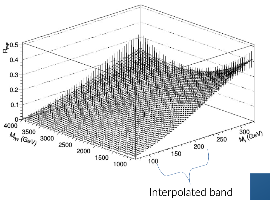
The figure below communicates how the various signal and background regions relate to each other though selections, and how (this particular) transfer function is defined from ratios of pass/fails in the regions.
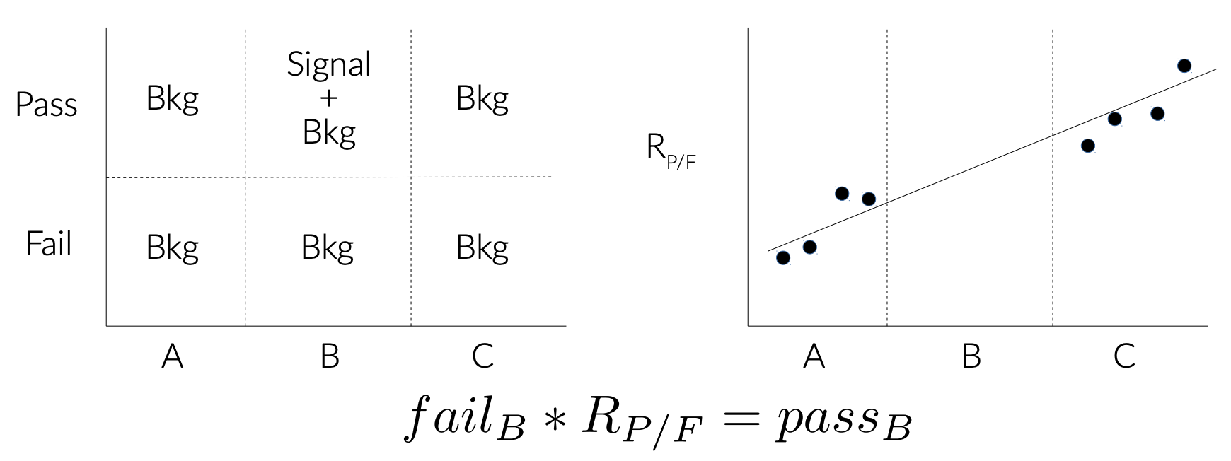
Question: What is the variable represented here by the x-axis? What do the regions A/B/C represent, and what the are selections dividing them? What does ‘pass’ and ‘fail’ refer to?
Solution
We can start with the pass/fail, which refers to the top tag. The x-axis is mtop, meaning the regions A/B/C are different mass ranges: A is low-mass, B is the top-mass window, and C is high-mass.
Need for Data Driven Background Estimation
QCD modeling is notoriusly hard to model. One strategy to modeling processes that are not well simulated is to remove the effect of well-modeled processes from data, then creating a shape template on which to match the poor-modeled background. This approach to estimating the background is called data-driven estimation.
Question: What background processes to our signal would be good candidates for data-driven estimation?
Solution
Multi-jet QCD is almost always estimated using a data-driven technique. In addition, the W+Jets process has a QCD-formed top candidates. ttbar and singletop are relatively well-modeled, however the normalization of their distributions are allowed to float in the final parameter fit.
Validation Regions
When we obtain either a scale factor or transfer function to extrapolate from the Control Region to the Signal Region, it is often useful to have a Validation Region that lies somewhere in between these two regions where one can apply the correction to the MC and check against data to ensure good agreement. In the framework we are walking you through, the fit uses all available (non-blinded) regions to simultaneously fit the transfer function parameters, leaing no space ‘between’ the SRs and CRs to define a VR.
Blinding
One thing to keep in mind when using data before settling on final signal and control region selections is the possibility of biasing one’s methods by being exposed to the data. For example, one could imagine a situation where one is ‘testing’ methods in a signal region and then observes a ‘problem’ (lack of events, too many events, etc) which guides the analyzer to biased decision-making. A similar problem can occur if a control or validation region is chosen that has significant signal contamination. To avoid these problems, we ‘blind’ our data whenever possible. That is, we do not look at any data in the SRs, when appropriate we could also deicde to remove data if it passes a significance threshold, and ensuring the control/validation regions have little signal contamination.
Key Points
The backgrounds involved are processes producing jets with large pT that look like t+W.
All-hadronic ttbar can look like t+W if one of tops has a very soft (or untagged) b-jet. MC is reasonably modeled
Singletop production is sub-dominant, but irreducible. MC is reasonably modeled
LHC is a hadron collider, multi-jet production (QCD) is almost always a background in all hadronic analyses.
W/Z+Jets behaves a lot like multi-jet production since the top-tag it passes to make it into out signal selection comes from combinatoric combination of jets.
Control regions are used to study specific backgrounds in a kinematic region orthogonal to the signal regions; we test our background estimation in CRs and apply corrections needed there to the SR.
Validation regions are designed to lie orthgonal but between CRs and SRs, perhaps with lower target BG purity, to test the corrections extracted from the CR that will be applied to SRs.
Blinding is the convention of not looking at data in the SR (or any signal-enriched selection).
Background Estimation: 2DAlphabet
Overview
Teaching: 10 min
Exercises: 50 minQuestions
How are we going to estimate the background?
What is 2DAlphabet?
Objectives
Familiarize with 2DAlphabet method
Recording files of this session are in cernbox
Idea of 2D Alphabet
Normally, we do a shape hunt along some observable and measure our background is near-by kintemtic regions to estimate its expected yield in the signal region. For our case, there is a clever way to do all these tasks simultaneously. Since we are scanning across mtW, with a window designated as a Signal Region, we can use all the non-window space to fit a smooth function that extrapolates over the SR window.
Since we define our SR as passing exactly one top tag (most importantly with a mass window cut), we can use the adjacent region of passing 2 top tags for a ttbar/singletop constrol region. We can then use the smooth function from above to estimate the multi-jet contribution to the 2-top measurement region. Whereas the multi-jet contribution’s shape is determined by the smooth function fit, the shape of the ttbar and singletop background is set by simulation and the normalization is allowed to float.
Simultaneous Fit
The fitting of the multi-jet background as well as the ttbar/singletop measurement are all done simultaneously. As the multijet estimation fit optimizes, the ttbar/singletop region feeds back its normalizations to subtract from the data used in the fit optimization. We also perform the fits separately but simultaneously across years (2016-2018). In summary, the fits are done on 3 years x 2 pass/fail x 2 multi-jet/ttbar (1/2-top) = 12 2D-regions (mt, mtW).
Exercise: Try Plotting CR and Get Familiar with 2DAlphabet
At tomorrow’s sessions you will dive into using 2DAlphabet for your own selections. For now, use the exisig code in BstarToTW_CMSDAS2020/examples/ex4.py to generate your own plots with selections meant for the ttbar and multi-jet CRs. You’ll need to mmodify the script and run the –select flag to make the new root files used for the plotting. As is, the script plots MC-only, can you add data to the CR plots?
Use the remaining time in the session to wrap up work in previous sessions, tomorrow we will run the 2DAlphabet framework to produce our limits. Also try looking into the 2DAlphabet framework to get an idea of how the code is structured and how you will change it tomorrow. Feel free to ask the facilitators any questions you have!
Key Points
We can simultaneously fit several backgrounds by defining the appropriate observables/axes, i.e. mt vs mtW.
2D Alphabet is a method of fitting a polynomial function to a space (except the SR), to model the multi-jet background, and also serves as an interfae to other tools.
Tuesday DAS Plenary 10-11h
Overview
Teaching: 60 min
Exercises: 0 minQuestions
Objectives
From 10-11h there will be a DAS Plenary, please tune in to that.
Key Points
Modelling the background and signal with 2DAlphabet (a wrapper for Combine)
Overview
Teaching: 30 min
Exercises: 40 minQuestions
How do I use the 2DAlphabet package to model the background?
Objectives
Run the 2DAlphabet package
Apply normalisation systematics
Apply shape systematics
Introduction to the 2DAlphabet package
2DAlphabet uses .json configuration files. Inside of these the are areas to add uncertainties which are used
inside of the combine backend. The 2DAlphabet serves as a nice interface with combine to allow the user to use
the 2DAlphabet method without having to create their own custom version of combine.
A look around
The configuration files that you will be using are located in the BstarToTW_CMSDAS2020 repository in this path BstarToTW_CMSDAS2020/configs_2Dalpha/
Take a look inside one of these files, for example: input_dataBsUnblind16.json
The options section contains boolean options, some of which are 2DAlphabet specific and others which map to combine.
Of the options the important ones to note are the blindedFit and blindedPlotswhich keep the signal regions blinded
and in a normal analysis would keep this option true until they reached the appropriate approval stage.
The process section is basically the same as the process section in combine, but laid out in an easier to read format.
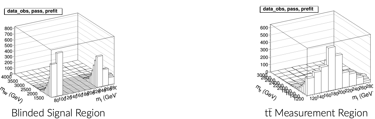
Each process refers to a root file containing data or Monte Carlo simulation. A "CODE" of 1 means that the process
is the data, a "CODE" of 2 means that the process is a background, and
a "CODE" of 0 means that a process is a signal event. The "SYSTEMATICS" list contains the names of the systematic
uncertainties for that process. The systematic uncertainties are assigned values in the "SYSTEMATIC" section. The
HISTPASS and HISTFAIL refer to the pass or fail bins of a histogram. The “PASS” bin indicates the signal region
whereas the “FAIL” bin indicates the multijet control region.
For more details on the sections in the configuration files, see the 2DAlphabet Documentation
Running 2DAlphabet
In order to run the 2DAlphabet package on our json configuration files, we will first make a symbolic link to the configuration files to make things easier.
# start inside the directory containing the BstarToTW_CMSDAS2020 repo
cd CMSSW_11_0_1/src/BstarToTW_CMSDAS2020/
# Now move to the directory containing the 2DAlphabet
cd ../../../CMSSW_10_6_14/src/2DAlphabet
# now create a symlink (symbolic link) to the config file directory
ln -s ../../../CMSSW_11_0_1/src/BstarToTW_CMSDAS2020/configs_2Dalpha/ configs_2Dalpha
Now run one of the configuration files.
cmsenv
# now run one of the files
python run_MLfit.py configs_2Dalpha/input_dataBsUnblind16.json --tag=bsTest
This will create some output plots and combine cards. The output is stored in bsTest/SR16/.
Tip
If running with the configuration files for all three years, you can append
--fullRun2and that will add together the 2016, 2017, and 2018 results for the signal region and ttbar measurement region separately so that there are fewer plots to view.
Uncertainties
There are two types of systematic uncertainties that can be added to combine: normalisation uncertainties and shape uncertainties. Since this is a simplified analysis, we consider two normalisation uncertainties (luminosity and cross section) and one shape uncertainty (Top pT re-weighting) with one optional bonus exercise.
Where to add the uncertainties
Let’s take a look at adding uncertainties in the .json files. The systematic uncertainties are defined in the SYSTEMATIC section:
"SYSTEMATIC": {
    "HELP": "All systematics should be configured here. The info for them will be pulled for each process that calls each systematic. These are classified by codes 0 (symmetric, lnN), 1 (asymmetric, lnN), 2 (shape and in same file as nominal), 3 (shape and NOT in same file as nominal)",
    "lumi16": {
        "CODE": 0,
        "VAL": 1.025
    },
So in our json file, we can list a systematic and use the "CODE" to describe the type of systematic that will be used in combine.
The help message describes the options. Here, lnN refers to log-normal normalisation uncertainty.
As an example take a closer look at the "lumi16" systematic. It is a symmetric uncertainty "VAL": 1.025. In this context,
"VAL" refers to effect that the systematic has. In this case 1.025 means that this systematic has a 2.5% uncertainty on the yield.
For the moment, let’s just look at our symmetric uncertainties and later we will look at a shape uncertainty.
Luminosity uncertainties
As we saw in the previous example, the luminosity is a symmetric uncertainty. Each year, the amount of data collected (“luminosity”) is measured. This measurement has some uncertainty which means the uncertainty changes for each year and is uncorrelated between the years.
Discuss (5 min)
Should each Monte Carlo sample have a different luminosity uncertainty?
Solution
Monte Carlo samples for the same year should all have the same luminosity uncertainty, because the overall luminosity delivered by the detector in that year is a fixed measurement.
Cross section uncertainties
The cross section uncertainty is another symmetric uncertainty added to each Monte Carlo sample.
Discuss (5 min)
Should the signal Monte Carlo sample have a cross section uncertainty?
Solution
No. This is because the “cross section” of the signal is exactly what we want to fit for (ie. the parameter of interest/POI/r/mu)! One might ask then why we assign an uncertainty from the luminosity to the signal when the luminosity is just another normalization uncertainty. The answer is that the luminosity uncertainty is fundamentally different from the cross section uncertainties because it is correlated across all of the processes - if it goes up for one, it goes up for all. The cross section uncertainties though are per-process - the ttbar cross section can go up and the single top contribution will remain the same.
With just the luminosity and cross section uncertainties, we only have normalization uncertainties accounted for and there are certainly uncertainties which affect the shapes of distributions (our simulation is not perfect in many ways). These can be accounted for via vertical template interpolation (also called “template morphing”). The high-level explanation is that you can provide an “up” shape and a “down” shape in addition to the “nominal” and the algorithm will map “up” to +1 sigma and “down” to -1 sigma on a Gaussian constraint. The first of these “shape” uncertainties is the Top pT uncertainty.
Top pT uncertainties
The TOP group has recommendations for how to account for consistent but not-understood disagreements in the top pT spectrum between ttbar simulation and ttbar in data (see this twiki for more information). This analysis falls into Case 3.1 from that twiki. The short version of the recommendation is that one should measure the top pT spectrum in a dedicated ttbar control region which is exactly what the ttbar measurement region of the analysis is for.
For this analysis the top jet mass window is 105-220 GeV which constrains the ttbar background but does not leave a lot of room to work with when blinded. Fortunately, mtt is correlated with top pT so we can just measure the correction in the 2D space while also fitting for QCD and all of the other systematics in the ttbar measurement region and signal region!
Bonus: Analysis details on decisions
The decision of the correction for the ttbar top pT spectrum was pretty simple. We just took the functional form (for POWHEG+Pythia8) farther down and rewrote it as e(α0.0615 - β0.0005*pT) where α and β are nominally 1 (so just the regular correction on that page). Then each α and β are individually varied to 0.5 and 1.5 to be our uncertainty templates for the vertical interpolation. These are what are assigned to Tpt-alpha and Tpt-beta. For example, if the post-fit value of Tpt-alpha was 1 and Tpt-beta was -1, the final effective form of our Tpt reweighting function would be e(1.50.0615 - 0.50.0005*pT).
Exercise (20 min)
Add the Top pT uncertainties to the appropriate processes and see the changes in combine.
The uncertainties are already included in the section on
"SYSTEMATICS". However, they have not been added to the individual processes. To start this exercise, add theTpt-alphaandTpt-betauncertainties to the appropriate processes. Which processes should these uncertainties be added to? Then add in the the uncertainties to the appropriate processes and rerun the 2DAlphabet. Compare the combine cards usingdiffto see the changes before and after adding in the top pT uncertainty.Do this exercise for
input_dataBsUnblind16.jsonand then after looking at the solution, apply to the other config files.Solution
The Top pT uncertainties should be applied to the
ttbarandttbar-semilepprocesses. For example:"ttbar": { "TITLE":"t#bar{t}", "FILE":"path/TWpreselection16_ttbar_tau32medium_ttbar.root", "HISTPASS":"MtwvMtPass", "HISTFAIL":"MtwvMtFail", "SYSTEMATICS":["lumi16","ttbar_xsec","Tpt-alpha","Tpt-beta"], "COLOR": 2, "CODE": 2 }Now, keep the data card made before doing this change and then run the code to see the difference.
# From the 2DAlphabet directory, store the old card
cp bsTest/SR16/card_SR16.txt no_topUn_SR16.txt
# Then, rerun the 2DAlphabet
python run_MLfit.py configs_2Dalpha/input_dataBsUnblind16.json --tag=bsTest
# Then look at the difference
diff no_topUn_SR16.txt bsTest/SR16/card_SR16.txt
To understand more about what is happening in combine and how this shape uncertainty is applied see this DAS exercise
Now that this change has been made for one process in one configuration file, apply the same change for all
ttbarandttbar-semilepprocesses in all 6 configuration files.Note that
ttbaris all-inclusive for 2016 and hadronic only for 2017 and 2018 so thettbar_semilepis included only in 2017 and 2018.
Bonus Exercise: Trigger Efficiency uncertainty
The trigger efficiency uncertainty is defined as a systematic in the configuration files. As a bonus exercise, add this shape systematic uncertainty to the processes. How do you measure Trigger efficiency? And how is this uncertainty calculated?
This exercise is a bonus and not necessary to continue on.
Key Points
Luminosity uncertainties affect all processes equally
Cross section uncertainties should not be applied to signal
Template morphing is used to determine shape uncertainties
Tuesday Lunch 12-13h
Overview
Teaching: 0 min
Exercises: 60 minQuestions
Objectives
Enjoy your lunch from 12-13h :)
Key Points
Obtaining upper cross section limits
Overview
Teaching: 10 min
Exercises: 50 minQuestions
How do we use the 2DAlphabet package to set limits?
Once I unblind, did we find new physics? If not, what can we say?
Objectives
Use the 2DAlphabet package to set limits
Provide expected sensitivity (upper cross-section limits) before unblinding as a function of resonance mass.
Unblind and compare observed to expected limits.
Limits!
This is one of the big milestones in an analysis, setting limits! After un-blinding the limit plot, you can see if you discovered new physics.
Running the limit setting program
The limit setting program for 2DAlphabet needs to be run for each mass point under consideration and for each year.
The fitting program must be run on each year before the limit program can be run. So make sure that you completed
the exercise from the Modeling exercise that uses run_MLfit.py.
Make Limits
First run the limit program for each of the mass points. There are 19 mass points between 1400 and 4000 (1400, 1600, …), so it might be a good idea for each of you to choose 4 mass points to do and then combine the results together.
python run_Limit.py configs_2Dalpha/input_data*.json --tag=LimitLH1400 --unblindData -d <name of dir from ML fit> signalLH2400:signalLH1400 --freezeFail
- The directory we used in the previous example was
bsTestso replace<name of dir from ML fit>withbsTest(or whatever you choose to name it).- tag is the name of the output directory.
- “signalLH2400:signalLH1400” allows us to find:replace any strigns in the configs (this is useful for swapping out one signal sample for another without having to write a new set of configs - in this case, “signalLH2400” is replaced with “signalLH1400”).
--freezeFailwhich will set the “fail” bins to their post-fit values and then make them constant.- optionally unblind with
--unblindData.python set_limit.py -s signals.txt --unblindThe
signals.txtfile uses commas and new lines to seperate the information. Here is an example for just three mass points.LimitLH1400, LimitLH1600, LimitLH1800 1400, 1600, 1800 0.7848, 0.3431, 0.1588 1.0, 0.1, 0.1Here are the meaning of the rows in order:
- Folder location where higgsCombineTest.AsymptoticLimits.mH120.root lives (this would be your –tag from the run_MLfit.py step)
- Mass in GeV
- Theoretical cross section for the theory line
- Normalized cross section (values stored in bstar_config.json)
Now use these steps to run the limit setting program on all 19 mass points.
Understanding the limits
Did you discover new physics? How do you know?
Key Points
We can define expected sensitivity of an analysis with simulation-only by assuming the data expected will be exactly what the background estimation predicts.
We combine the systematic variations as a 1/2-sigma envelope around nominal expectation to quantify the confidence of our measurement.
After unblinding, if we have a down-fluctuation of data the expected exclusion appears stronger and vice-versa with up-fluctuations and apparently weak exclusions.
Bonus: Calibrating a jet subtructure tagger.
Overview
Teaching: 15 min
Exercises: 45 minQuestions
How can I validate a jet substructure tagger in data?
What can be done if a tagger (object-selection technique) performs differently in data vs simulation?
Objectives
Implement a selection that is enriched in boosted W bosons and top quarks.
Extract efficiency scale factors.
Key Points
We can define tagger scale factors by measuring the efficiency of the tagger in t+W enriched regions.
DAS Presentations
Overview
Teaching: 0 min
Exercises: 300 minQuestions
Objectives
Get your presentations together and show the rest of DAS what you’ve been working on!
Key Points